Creating a consistent environment #
Reproducibility #
Now that we have had a bit of an introduction to how RStudio works and how we can manipulate data and make some plots, it’s time to get a bit more advanced.
One key component of working as a group on data science projects is reproducibility. This means that if you run the same code on multiple computers, you will get the same result.
The ability to recreate analyses depends on several factors, starting with the operating system and going down to specific version of packages that are used within R.
To control the operating system and all the complexities that come with eg Windows versus Mac, we will utilize Docker.
Docker #
For our purposes, Docker is a system that lets us run a second operating system within our computer. This second operating system can be started and stopped whenever we want. Importantly, this second operating system will ensure that we have the exact same computing environment across computers and people regardless of what kind of laptop or Desktop someone uses. Docker (or the related software Singularity) even scales to the level of cloud or cluster computing, allowing you to ensure you are always working with the same set of starting conditions.
Two things to understand about Docker at this point:
- An “image” is a description of the environment that we want to run
- A “container” is the environment itself. It can be started, stoppped and paused
Install Docker #
The first thing we will do is install Docker Desktop. It can be install for free from here.
Once this is setup, it will look something like this:
Pulling the lab image #
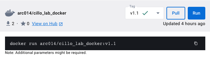
After you have installed Docker Desktop, the next thing to do is to pull the Cillo Lab docker image. This image contains a base linux installation with all the associated packages need to run RStudio and create output files from RMarkdown.
To find this image, simply type in “cillo_lab_docker” in the search bar at the top and click Pull. It should look something like this:
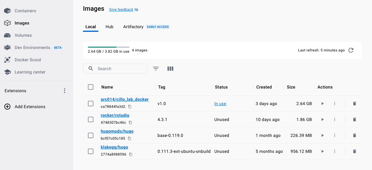
Once you have pulled this image, you can find it under you local Images by clicking the “Images” tab in the column on the left hand side of the user interface.
Setting up and starting the image #
Now that we have the image, we will start it. A few things to understand before we do so:
- Starting the image creates a container, which is basically a “sandbox” that is self-contained from which we will run RStudio
- We will have to use a port to access our self-contained operating system. This means that we will use RStudio through the browser (eg Google Chrome) instead of using the RStudio app as we did previously
- Containers do not automatically have access to any directories on your computer (since they are self contained). However, we want to be able to pass files back and forth from our normal computer to our virtual computer, so we will bind a directory
- We also want al the R libaries that we use to persist from one session to another in our container. To achieve this, we will put the R packages we download into specific directory that is shared with our normal computer and we will tell RStudio to use that directory to install and load packages
If this all sounds like non-sense, no worries! It will hopefully be much clearer once we walk through how to get the container up and running.
Starting a container with the right options #
Once we hit the play button under Actions from the Images tab, it will open up a screen that allows us to specify additional settings before clicking “Run”.
Open up the “Optional Settings” by clicking the down arrow, and you’ll see the following:
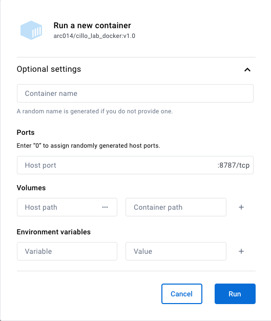
Add the following info:
- Container name: leave this blank, Docker usually picks far better names than we can come up with
- Ports: we will need to know which port to open in our browser after we start the container. It can be any open port, but I usually select something like “8888”
- Volumes: this is where we will bind the directory on our local computer to that on the virtual environment. For host path (the path from your normal computer), create a directory somewhere that you can easily find it and input it here. Bind this to the following container path “/home/rstudio/{whatever_you_named_your_directory}”. Make sure you didn’t use spaces in the directory name your created.
- Environment variables: Here is where we tell our virtual environment where to store and find packages. Let’s make a subdirectory in {whatever_you_named_your_directory} called “rlibs_to_use”. This will be where we store and load our libraries from. To tell RStudio to do so, add the following two environment variables and values:
- Variable = R_LIBS ; Value = /home/rstudio/{whatever_you_named_your_directory}/rlibs_to_use
- Variable = R_LIBS_USER ; Value = /home/rstudio/{whatever_you_named_your_directory}/rlibs_to_use
Finally, click run and Docker will start your container.
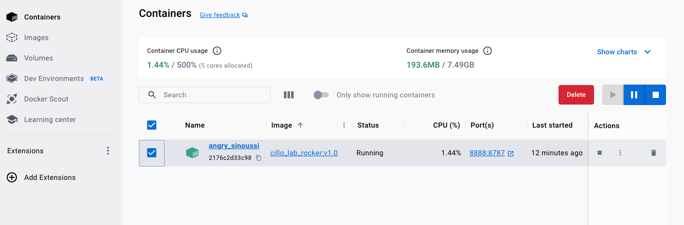
Once it’s running, if you open the Containers tab from the far left column, you’ll see the following:

Opening RStudio in the container #
The last thing we will do is open the version of RStudio that is running in the container. To achieve this, we will open our web browser and type the following:
http://localhost:8888
This opens the following window:
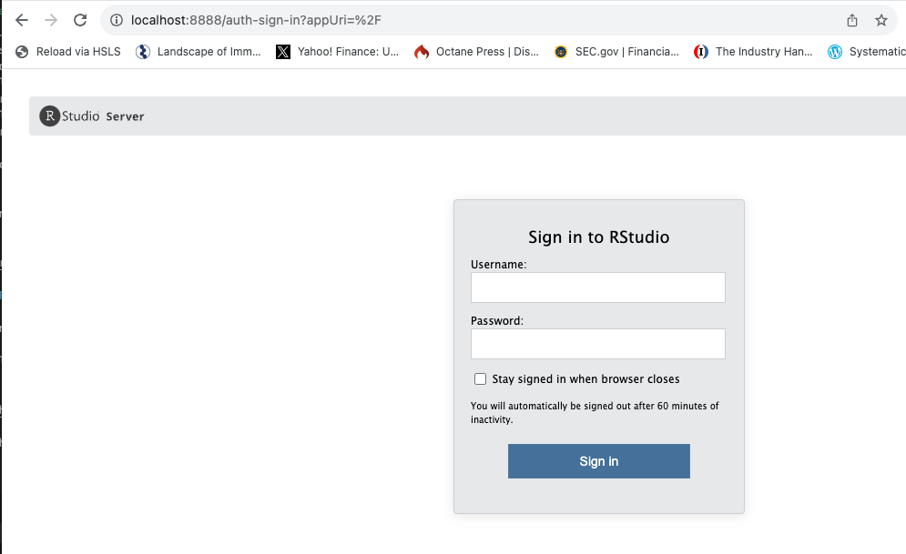
We can then put in the default username “rstudio”. The password can be found in the “Logs” section of the running container. If this does not automatically open when you start the container, you can navigate there by clicking on the name of the running container.
The password assigned for this RStudio container should be listed there. My screen looks like this:
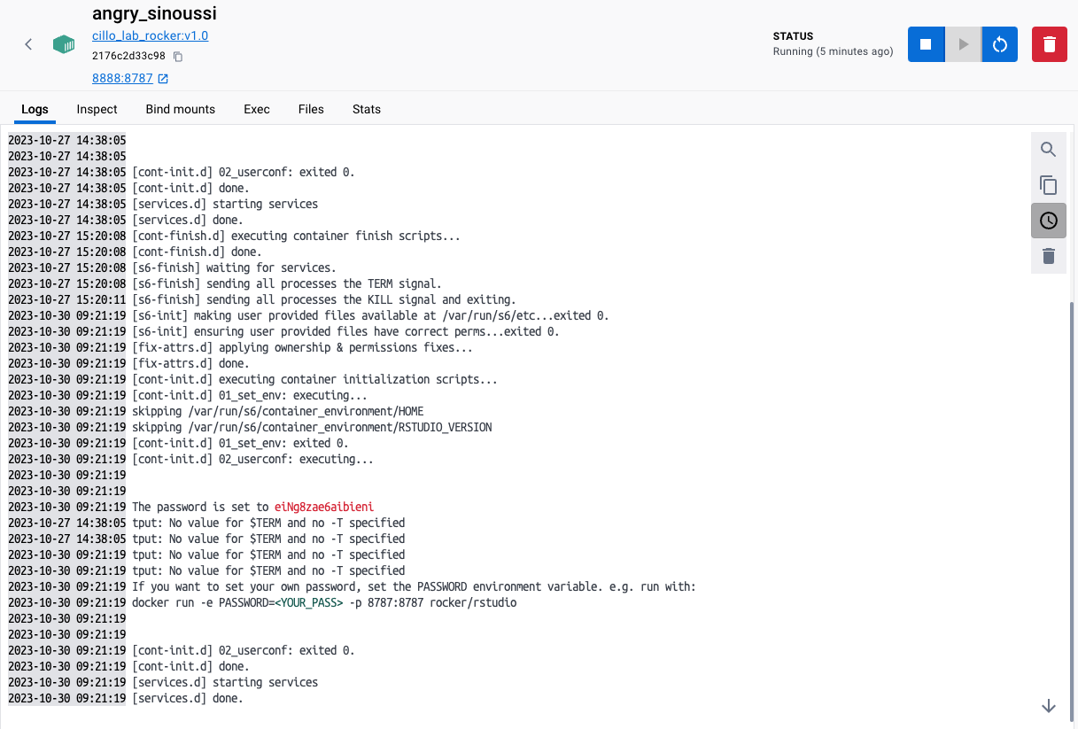
And you can see the password generated for my session is “eiNg8zae6aibieni”. Really rolls of the tongue.
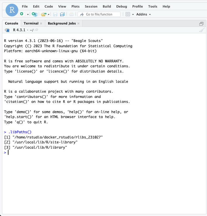
Checking the Volumes mounted appropriately #
Log in to RStudio, and in the command line type the following:
“.libPaths()”
Which will return several items, the first of which should be the path to the directory that we specified for hold our libraries.
Using RStudio #
Now, you can use RStudio just like on your Desktop. The only caveat is that any files that you save or want to open in this “dockerized” RStudio need to be present in the mounted directory, i.e. /home/rstudio/{whatever_you_named_your_directory} in your RStudio container and the directory you assigned from your computer.
These two directories are mirrored, so whatever you do from either your computer of the Docker container is saved. Since we mounted the directory from our local computer, this will save all the files even if/when you kill the container.
Stopping the container #
You can stop the container by clicking the stop button when the container is selected in the Containers window.
It’s a good idea to stop the container when you aren’t using it because running a second operating system on your computer is resource intensive (i.e. will slow down your computer if you are trying to do other things and will kill you battery if you aren’t plugged in).
If you stop the container, you can restart it later and pick up where you left off without having to mess around with specifying all the options again.
Alternatively, if you are feeling spiteful you can delete the container entirely. But if you want to start it again, you have to go back to the image and input all the optional goodies again.
Conclusions #
Congrats if you made it this far! You now have a fully reproducible environment from which you can do all your analysis.
This is really only scratching the surface of what you can do with Docker, but it suits our needs!