RMarkdown #

There are often two challenges with any significant science project:

Reproducibility, which we have partially tackled with Docker in the previous post
Communication of results

We will use RMarkdown to address both of these challenges, which are particularly acute in data science and computational biology projects. RMarkdown allows us to blend code and output into a single file. This is a major advance over either typing code directly in the R console or even writing scripts that we then execute with R. The reason for this is that RMarkdown allows us to see the code and its output in the same place. This also provides reproducibility, as someone reading you code later will be able to reproduce it AND determine if the output is the same with relative ease.

This tutorial will be a concise guide to RMarkdown, but there is a lot more that we can do with it than we will cover here. The interested reader should refer to this excellent Bookdown guide by Yihue Xie, JJ Allaire and Garrett Grolemund. Another great resource is knitr in a nutshell by Karl Broman.

Under the hood, R Markdown is using knitr and Pandoc to convert the R Markdown document to a different format (such as a PDF or in this case an HTML). The nice thing is that RStudio abstracts away all the nuts and bolts of this process.

Getting started #

To get started, we will first open up RStudio (either locally or through a Docker instance). We can then create a blank RMarkdown document by going to:

File > New File > R Markdown…

I’ll note that there are other formats available here too much as R Notebooks and Quarto. Quarto, in particular, is becoming more popular and may one day overtake RMarkdown. But for now, we will be sticking with RMarkdown.

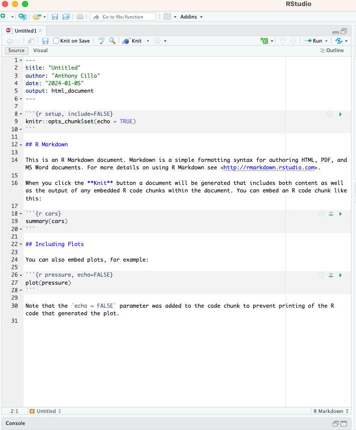
Once you have created a new R Markdown document, you will have a template to get started that looks like this:

Front matter #

At the top of the document, you’ll see a header section that has title, author, date and output by default. This region can be used to change these values to suit your needs. One thing that’s nice is you can also use variables or R code here. For example, you can change the date to “Sys.Date()” which will automatically output the current date.

Code blocks #

The next thing of interest are the regions that start with 3 backticks and end with 3 backticks. These are called code blocks, and are nice ways to discretely package your code into manageable chunks (i.e. chunks that accomplish a specific goal).

The only thing that is required to create an R code block is the following: “```{r}”. But, it’s also good practice to succinctly name the code blocks, generally by the goal they are accomplishing. In the template, you can see the second code block is called cars.

You can also specify different features for the code block following the initial set of backticks. In the template, you can see that “include=FALSE” is present, which prevents that code block from being part of the final document when it’s rendered (see below for info about rendering).

Finally, you can see in the first code block that you can also set global options for the entire document using knitr. In this case, we are setting echo to TRUE for all code blocks, which will print the code followed by it’s output in the final document. Generally, we don’t need to mess with an knitr settings for a nice output.

Writing a code block #

Often, in the first code block I like to load all the packages we will need for downstream analyses. In this case, we are just going to load Tidyverse to create a few example plots for the toy dataset mpg.

Note that the here package is being used to automatically set up a path to the folder that contains to RMD file that we are creating. This is useful for keeping track of the files that are generated during the course of a project.

library(tidyverse)

    ## ── Attaching core tidyverse packages ──────────────────────── tidyverse 2.0.0 ──
    ## ✔ dplyr     1.1.2     ✔ readr     2.1.4
    ## ✔ forcats   1.0.0     ✔ stringr   1.5.0
    ## ✔ ggplot2   3.4.4     ✔ tibble    3.2.1
    ## ✔ lubridate 1.9.2     ✔ tidyr     1.3.0
    ## ✔ purrr     1.0.2     
    ## ── Conflicts ────────────────────────────────────────── tidyverse_conflicts() ──
    ## ✖ dplyr::filter() masks stats::filter()
    ## ✖ dplyr::lag()    masks stats::lag()
    ## ℹ Use the conflicted package (<http://conflicted.r-lib.org/>) to force all conflicts to become errors

library(here)

    ## here() starts at /Users/ARC85/Desktop/rmd_tutorial

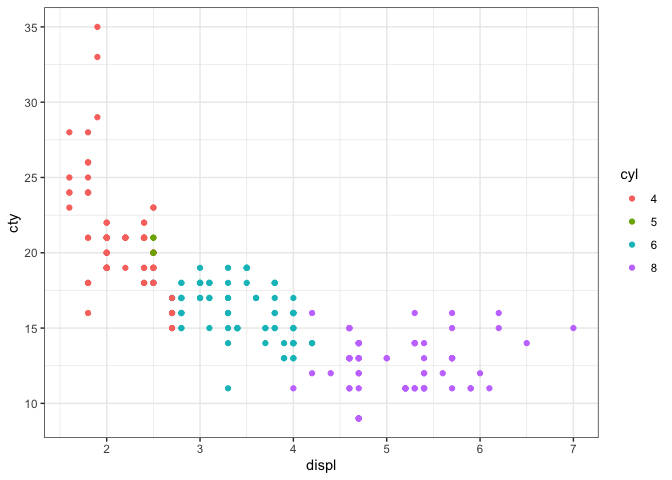
Create a plot #

Here, we’re just creating a plot in a code block.

mpg %>%
  mutate(cyl=as.factor(cyl)) %>%
  ggplot(.,aes(x=displ,y=cty,colour=cyl)) +
  geom_point() +
  theme_bw()

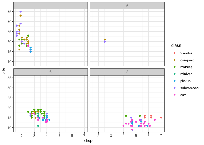
Create a plot #

We’re going to create another plot, but use the echo=FALSE feature when defining the code chunk. This means that only the plot will appear and the code used to create it will be hidden.

Save output #

saveRDS(mpg,file=here("mpg_data.rds"))

Knitting the document #

The final step of doing an analysis in RMarkdown is creating the output file. This process is called “knitting” the document. The easiest way to do this is to click the knit button at the top of the page and click “Knit to HTML” from the dropdown menu. That’s it - now you have a nice HTML file to document and communicate your analysis.