
Intro to scRNAseq analysis #
This intro is will guide you through a very simple analysis of 2,700 peripheral blood mononuclear cells from a healthy donor. The full tutorial can be found here, but I have cherry-picked what I deem to be the most important components for our purposes.
In general, the workflow follows these steps:
- Read in data
- Normalize count data for library size
- Find variable features
- Reduce dimensionality
- Find Clusters
- Plot UMAPs
- Find differentially expressed genes
- Identify cell types
- Downstream biological analyses
- Other analyses or modeling
Background #
These healthy donor cells were generated using 10X Genomics 3’-based single-cell RNAseq platform. The libaries were contructed and sequenced on a NextSeq500. CellRanger was used to align the reads from the NextSeq500 to the human genome reference, identify genes, count genes, and assign counts to unique molecular identifiers to build a feature barcode matrix. Generating the feature barcode matrix will be outlined in a future tutorial since it requires command line coding.
Most critially: this feature barcode matrix will serve as our input to Seurat. This analysis only has 1 feature barcode matrix, but more complex analyses often have more than one feature barcode matrix that must be combined for downstream analyses.
Prerequisites #
Before we get started with this analysis, we need to download the feature barcode matrix. This matrix is publicly available from 10X Genomics and can be downloaded here.
Place this file in a location that you can access easily via R. In this example, we will assume I have the data file in my working directory.
Load packages #
First, we will load the necessary packages.
library(Seurat)
library(dplyr) # from the tidyverse
library(patchwork) # for combining ggplots
Create a Seurat object #
Next, we will load the raw data and create a Seurat object from it.
# Read in the data
pbmc_data <- Read10X("~/Desktop/pbmc3k_vignette/pbmc3k/filtered_gene_bc_matrices/hg19")

# Check out the data - it's a sparse matrix
pbmc_data[1:10,1:10]
    ## 10 x 10 sparse Matrix of class "dgCMatrix"

    ##   [[ suppressing 10 column names 'AAACATACAACCAC-1', 'AAACATTGAGCTAC-1', 'AAACATTGATCAGC-1' ... ]]
    ##
    ## MIR1302-10    . . . . . . . . . .
    ## FAM138A       . . . . . . . . . .
    ## OR4F5         . . . . . . . . . .
    ## RP11-34P13.7  . . . . . . . . . .
    ## RP11-34P13.8  . . . . . . . . . .
    ## AL627309.1    . . . . . . . . . .
    ## RP11-34P13.14 . . . . . . . . . .
    ## RP11-34P13.9  . . . . . . . . . .
    ## AP006222.2    . . . . . . . . . .
    ## RP4-669L17.10 . . . . . . . . . .
# Look at some specific genes
pbmc_data[c("CD3D", "TCL1A", "MS4A1"), 1:30]
    ## 3 x 30 sparse Matrix of class "dgCMatrix"

    ##   [[ suppressing 30 column names 'AAACATACAACCAC-1', 'AAACATTGAGCTAC-1', 'AAACATTGATCAGC-1' ... ]]

    ##
    ## CD3D  4 . 10 . . 1 2 3 1 . . 2 7 1 . . 1 3 . 2  3 . . . . . 3 4 1 5
    ## TCL1A . .  . . . . . . 1 . . . . . . . . . . .  . 1 . . . . . . . .
    ## MS4A1 . 6  . . . . . . 1 1 1 . . . . . . . . . 36 1 2 . . 2 . . . .
# Create a Seurat object from the data
pbmc_ser <- CreateSeuratObject(counts=pbmc_data,project="pbmc3k",min.cells=3,min.features=200)
    ## Warning: Feature names cannot have underscores ('_'), replacing with dashes
    ## ('-')
# Check out the constructed Seurat object
pbmc_ser
    ## An object of class Seurat
    ## 13714 features across 2700 samples within 1 assay
    ## Active assay: RNA (13714 features, 0 variable features)
# Metadata is automatically generated and can be viewed
head(pbmc_ser@meta.data)
    ##                  orig.ident nCount_RNA nFeature_RNA
    ## AAACATACAACCAC-1     pbmc3k       2419          779
    ## AAACATTGAGCTAC-1     pbmc3k       4903         1352
    ## AAACATTGATCAGC-1     pbmc3k       3147         1129
    ## AAACCGTGCTTCCG-1     pbmc3k       2639          960
    ## AAACCGTGTATGCG-1     pbmc3k        980          521
    ## AAACGCACTGGTAC-1     pbmc3k       2163          781
Quality control and filtering #
Prior to beginning any analysis, we need to perform a quality control across the dataset.
Commonly used criteria for QC are: 1) Low number of unique genes per cell - low number of genes and/or counts likely means that the cell was ruptured or dying during library generation and should be removed. 2) Percentage of genes aligning to mitochondrial reads per cell - a high frequency of mitochondrial reads per cell also indicates poor cell quality during library generation
Any cells outside of these criteria should be excluded.
It’s important to always use dataset specific cutoffs (rather than general cutoffs) because these values depend on the species, cell types, and sequencing depth of any given experiment.
Note that mitochondrial genes can be identified as starting with “MT-”.
# The [[ ]] operator can add columns to object metadata. This is a great place to stash QC stats
pbmc_ser[["percent_mt"]] <- PercentageFeatureSet(pbmc_ser, pattern = "^MT-")

# Check out metadata now
head(pbmc_ser@meta.data)
    ##                  orig.ident nCount_RNA nFeature_RNA percent_mt
    ## AAACATACAACCAC-1     pbmc3k       2419          779  3.0177759
    ## AAACATTGAGCTAC-1     pbmc3k       4903         1352  3.7935958
    ## AAACATTGATCAGC-1     pbmc3k       3147         1129  0.8897363
    ## AAACCGTGCTTCCG-1     pbmc3k       2639          960  1.7430845
    ## AAACCGTGTATGCG-1     pbmc3k        980          521  1.2244898
    ## AAACGCACTGGTAC-1     pbmc3k       2163          781  1.6643551
# We can also plot values from metadata
VlnPlot(pbmc_ser, features = c("nFeature_RNA", "nCount_RNA", "percent_mt"), ncol = 3)
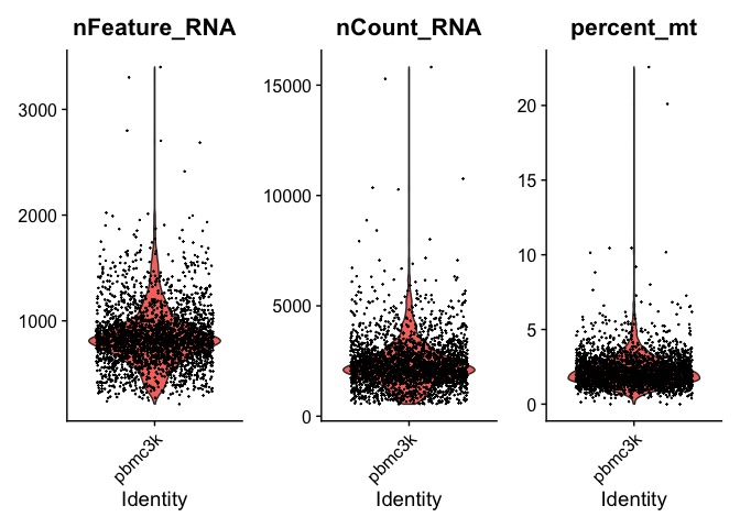
# We will filter to cells with greater than 200 genes and less than 2500 genes
# We will also exclude cells with greater than 5% MT reads
pbmc_ser <- subset(pbmc_ser, subset = nFeature_RNA > 200 & nFeature_RNA < 2500 & percent_mt < 5)
Normalization #
pbmc_ser <- NormalizeData(pbmc_ser, normalization.method = "LogNormalize", scale.factor = 10000)
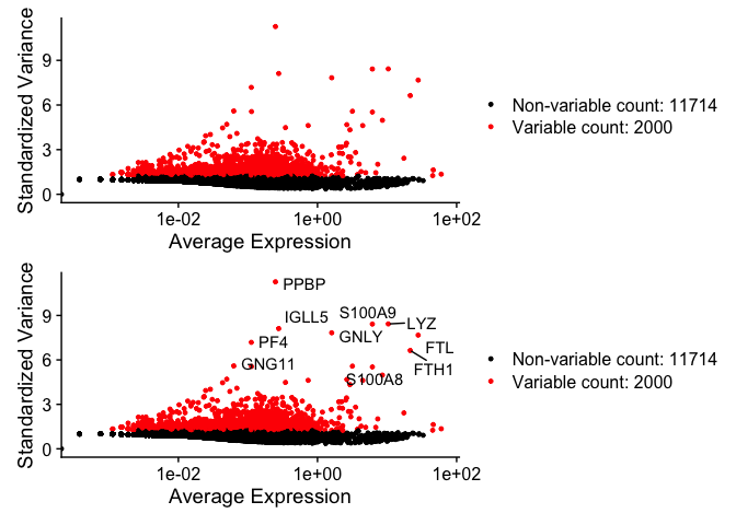
Identify highly variable features #
pbmc_ser <- FindVariableFeatures(pbmc_ser, selection.method = "vst", nfeatures = 2000)

# Identify the 10 most highly variable genes
top10 <- head(VariableFeatures(pbmc_ser), 10)

# plot variable features with and without labels
plot1 <- VariableFeaturePlot(pbmc_ser)
plot2 <- LabelPoints(plot = plot1, points = top10, repel = TRUE)

## When using repel, set xnudge and ynudge to 0 for optimal results

plot1 / plot2
    ## Warning: Transformation introduced infinite values in continuous x-axis
    ## Transformation introduced infinite values in continuous x-axis
Scale data and reduce dimensionality #
pbmc_ser <- ScaleData(pbmc_ser)

## Centering and scaling data matrix

pbmc_ser <- RunPCA(pbmc_ser, features = VariableFeatures(object = pbmc_ser))
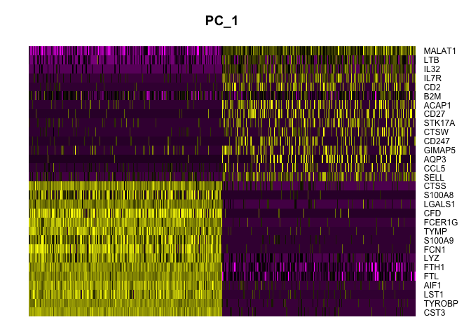
    ## PC_ 1
    ## Positive:  CST3, TYROBP, LST1, AIF1, FTL, FTH1, LYZ, FCN1, S100A9, TYMP
    ##     FCER1G, CFD, LGALS1, S100A8, CTSS, LGALS2, SERPINA1, IFITM3, SPI1, CFP
    ##     PSAP, IFI30, SAT1, COTL1, S100A11, NPC2, GRN, LGALS3, GSTP1, PYCARD
    ## Negative:  MALAT1, LTB, IL32, IL7R, CD2, B2M, ACAP1, CD27, STK17A, CTSW
    ##     CD247, GIMAP5, AQP3, CCL5, SELL, TRAF3IP3, GZMA, MAL, CST7, ITM2A
    ##     MYC, GIMAP7, HOPX, BEX2, LDLRAP1, GZMK, ETS1, ZAP70, TNFAIP8, RIC3
    ## PC_ 2
    ## Positive:  CD79A, MS4A1, TCL1A, HLA-DQA1, HLA-DQB1, HLA-DRA, LINC00926, CD79B, HLA-DRB1, CD74
    ##     HLA-DMA, HLA-DPB1, HLA-DQA2, CD37, HLA-DRB5, HLA-DMB, HLA-DPA1, FCRLA, HVCN1, LTB
    ##     BLNK, P2RX5, IGLL5, IRF8, SWAP70, ARHGAP24, FCGR2B, SMIM14, PPP1R14A, C16orf74
    ## Negative:  NKG7, PRF1, CST7, GZMB, GZMA, FGFBP2, CTSW, GNLY, B2M, SPON2
    ##     CCL4, GZMH, FCGR3A, CCL5, CD247, XCL2, CLIC3, AKR1C3, SRGN, HOPX
    ##     TTC38, APMAP, CTSC, S100A4, IGFBP7, ANXA1, ID2, IL32, XCL1, RHOC
    ## PC_ 3
    ## Positive:  HLA-DQA1, CD79A, CD79B, HLA-DQB1, HLA-DPB1, HLA-DPA1, CD74, MS4A1, HLA-DRB1, HLA-DRA
    ##     HLA-DRB5, HLA-DQA2, TCL1A, LINC00926, HLA-DMB, HLA-DMA, CD37, HVCN1, FCRLA, IRF8
    ##     PLAC8, BLNK, MALAT1, SMIM14, PLD4, P2RX5, IGLL5, LAT2, SWAP70, FCGR2B
    ## Negative:  PPBP, PF4, SDPR, SPARC, GNG11, NRGN, GP9, RGS18, TUBB1, CLU
    ##     HIST1H2AC, AP001189.4, ITGA2B, CD9, TMEM40, PTCRA, CA2, ACRBP, MMD, TREML1
    ##     NGFRAP1, F13A1, SEPT5, RUFY1, TSC22D1, MPP1, CMTM5, RP11-367G6.3, MYL9, GP1BA
    ## PC_ 4
    ## Positive:  HLA-DQA1, CD79B, CD79A, MS4A1, HLA-DQB1, CD74, HIST1H2AC, HLA-DPB1, PF4, SDPR
    ##     TCL1A, HLA-DRB1, HLA-DPA1, HLA-DQA2, PPBP, HLA-DRA, LINC00926, GNG11, SPARC, HLA-DRB5
    ##     GP9, AP001189.4, CA2, PTCRA, CD9, NRGN, RGS18, CLU, TUBB1, GZMB
    ## Negative:  VIM, IL7R, S100A6, IL32, S100A8, S100A4, GIMAP7, S100A10, S100A9, MAL
    ##     AQP3, CD2, CD14, FYB, LGALS2, GIMAP4, ANXA1, CD27, FCN1, RBP7
    ##     LYZ, S100A11, GIMAP5, MS4A6A, S100A12, FOLR3, TRABD2A, AIF1, IL8, IFI6
    ## PC_ 5
    ## Positive:  GZMB, NKG7, S100A8, FGFBP2, GNLY, CCL4, CST7, PRF1, GZMA, SPON2
    ##     GZMH, S100A9, LGALS2, CCL3, CTSW, XCL2, CD14, CLIC3, S100A12, RBP7
    ##     CCL5, MS4A6A, GSTP1, FOLR3, IGFBP7, TYROBP, TTC38, AKR1C3, XCL1, HOPX
    ## Negative:  LTB, IL7R, CKB, VIM, MS4A7, AQP3, CYTIP, RP11-290F20.3, SIGLEC10, HMOX1
    ##     LILRB2, PTGES3, MAL, CD27, HN1, CD2, GDI2, CORO1B, ANXA5, TUBA1B
    ##     FAM110A, ATP1A1, TRADD, PPA1, CCDC109B, ABRACL, CTD-2006K23.1, WARS, VMO1, FYB
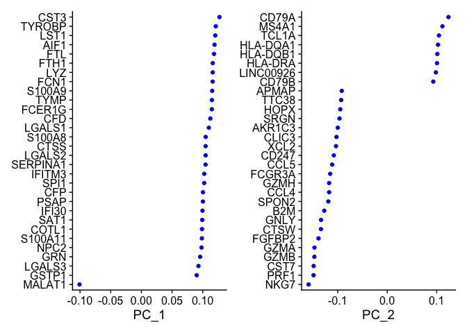
Check out reduced dimensions in PCA space #
print(pbmc_ser[["pca"]], dims = 1:5, nfeatures = 5)
    ## PC_ 1
    ## Positive:  CST3, TYROBP, LST1, AIF1, FTL
    ## Negative:  MALAT1, LTB, IL32, IL7R, CD2
    ## PC_ 2
    ## Positive:  CD79A, MS4A1, TCL1A, HLA-DQA1, HLA-DQB1
    ## Negative:  NKG7, PRF1, CST7, GZMB, GZMA
    ## PC_ 3
    ## Positive:  HLA-DQA1, CD79A, CD79B, HLA-DQB1, HLA-DPB1
    ## Negative:  PPBP, PF4, SDPR, SPARC, GNG11
    ## PC_ 4
    ## Positive:  HLA-DQA1, CD79B, CD79A, MS4A1, HLA-DQB1
    ## Negative:  VIM, IL7R, S100A6, IL32, S100A8
    ## PC_ 5
    ## Positive:  GZMB, NKG7, S100A8, FGFBP2, GNLY
    ## Negative:  LTB, IL7R, CKB, VIM, MS4A7
VizDimLoadings(pbmc_ser, dims = 1:2, reduction = "pca")
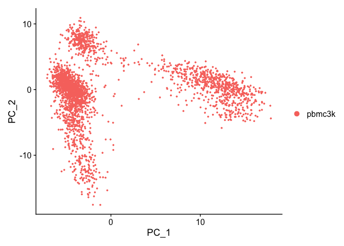
DimPlot(pbmc_ser, reduction = "pca")
DimHeatmap(pbmc_ser, dims = 1, cells = 500, balanced = TRUE)
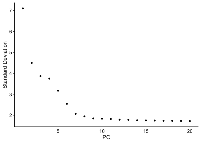
ElbowPlot(pbmc_ser)
Cluster cells #
pbmc_ser <- FindNeighbors(pbmc_ser, dims = 1:7)
    ## Computing nearest neighbor graph

    ## Computing SNN

    pbmc_ser <- FindClusters(pbmc_ser, resolution = c(0.3,0.5,0.7))

    ## Modularity Optimizer version 1.3.0 by Ludo Waltman and Nees Jan van Eck
    ##
    ## Number of nodes: 2638
    ## Number of edges: 88288
    ##
    ## Running Louvain algorithm...
    ## Maximum modularity in 10 random starts: 0.9150
    ## Number of communities: 9
    ## Elapsed time: 0 seconds
    ## Modularity Optimizer version 1.3.0 by Ludo Waltman and Nees Jan van Eck
    ##
    ## Number of nodes: 2638
    ## Number of edges: 88288
    ##
    ## Running Louvain algorithm...
    ## Maximum modularity in 10 random starts: 0.8827
    ## Number of communities: 10
    ## Elapsed time: 0 seconds
    ## Modularity Optimizer version 1.3.0 by Ludo Waltman and Nees Jan van Eck
    ##
    ## Number of nodes: 2638
    ## Number of edges: 88288
    ##
    ## Running Louvain algorithm...
    ## Maximum modularity in 10 random starts: 0.8576
    ## Number of communities: 11
    ## Elapsed time: 0 seconds
dplyr::glimpse(pbmc_ser@meta.data)
    ## Rows: 2,638
    ## Columns: 8
    ## $ orig.ident      <fct> pbmc3k, pbmc3k, pbmc3k, pbmc3k, pbmc3k, pbmc3k, pbmc3k…
    ## $ nCount_RNA      <dbl> 2419, 4903, 3147, 2639, 980, 2163, 2175, 2260, 1275, 1…
    ## $ nFeature_RNA    <int> 779, 1352, 1129, 960, 521, 781, 782, 790, 532, 550, 11…
    ## $ percent_mt      <dbl> 3.0177759, 3.7935958, 0.8897363, 1.7430845, 1.2244898,…
    ## $ RNA_snn_res.0.3 <fct> 2, 3, 2, 1, 6, 2, 4, 4, 0, 5, 3, 0, 0, 1, 0, 0, 1, 2, …
    ## $ RNA_snn_res.0.5 <fct> 1, 2, 1, 4, 7, 1, 3, 3, 3, 6, 2, 0, 0, 4, 3, 0, 4, 1, …
    ## $ RNA_snn_res.0.7 <fct> 5, 2, 1, 4, 8, 1, 3, 3, 5, 7, 2, 0, 0, 4, 5, 5, 4, 1, …
    ## $ seurat_clusters <fct> 5, 2, 1, 4, 8, 1, 3, 3, 5, 7, 2, 0, 0, 4, 5, 5, 4, 1, …
Idents(pbmc_ser) <- "RNA_snn_res.0.3"
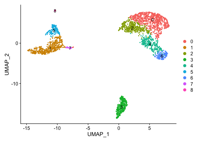
Create UMAP for visualization #
# If you haven't installed UMAP, you can do so via reticulate::py_install(packages = 'umap-learn')

pbmc_ser <- RunUMAP(pbmc_ser, dims = 1:7)
    ## 22:20:58 UMAP embedding parameters a = 0.9922 b = 1.112

    ## 22:20:58 Read 2638 rows and found 7 numeric columns

    ## 22:20:58 Using Annoy for neighbor search, n_neighbors = 30

    ## 22:20:58 Building Annoy index with metric = cosine, n_trees = 50

    ## 0%   10   20   30   40   50   60   70   80   90   100%

    ## [----|----|----|----|----|----|----|----|----|----|

    ## **************************************************|
    ## 22:20:58 Writing NN index file to temp file /var/folders/1w/32zp8ffj6q50nny8nt6y1bvc0000gq/T//Rtmpfk3bAq/file75b87017f822
    ## 22:20:58 Searching Annoy index using 1 thread, search_k = 3000
    ## 22:20:58 Annoy recall = 100%
    ## 22:20:58 Commencing smooth kNN distance calibration using 1 thread with target n_neighbors = 30
    ## 22:20:59 Initializing from normalized Laplacian + noise (using irlba)
    ## 22:20:59 Commencing optimization for 500 epochs, with 102208 positive edges
    ## 22:21:01 Optimization finished
DimPlot(pbmc_ser, reduction = "umap",label=T)
Evaluating differentially expressed genes #
# find all markers of cluster 2
cluster2_markers <- FindMarkers(pbmc_ser, ident.1 = 2, min.pct = 0.25)
head(cluster2_markers, n = 5)
    ##             p_val avg_log2FC pct.1 pct.2    p_val_adj
    ## IL32 1.400312e-82  1.2326710 0.960 0.480 1.920389e-78
    ## LTB  9.486821e-76  1.2798994 0.982 0.654 1.301023e-71
    ## AQP3 1.191119e-59  1.3174581 0.451 0.117 1.633501e-55
    ## IL7R 5.609743e-57  1.1300879 0.759 0.339 7.693202e-53
    ## CD3D 1.279636e-56  0.8208297 0.920 0.449 1.754893e-52
# find all markers distinguishing cluster 5 from clusters 0 and 3
cluster5_markers <- FindMarkers(pbmc_ser, ident.1 = 5, ident.2 = c(0, 3), min.pct = 0.25)
head(cluster5_markers, n = 5)
    ##                       p_val avg_log2FC pct.1 pct.2     p_val_adj
    ## FCGR3A        2.497558e-219   4.272442 0.975 0.038 3.425151e-215
    ## IFITM3        3.174718e-210   3.892867 0.975 0.045 4.353808e-206
    ## CFD           2.902241e-205   3.407246 0.938 0.038 3.980133e-201
    ## CD68          9.447858e-205   3.024369 0.926 0.034 1.295679e-200
    ## RP11-290F20.3 3.102169e-202   2.728929 0.840 0.015 4.254314e-198
# find markers for every cluster compared to all remaining cells, report only the positive ones
pbmc_markers <- FindAllMarkers(pbmc_ser, only.pos = TRUE, min.pct = 0.25, logfc.threshold = 0.25)
    ## Calculating cluster 0

    ## Calculating cluster 1

    ## Calculating cluster 2

    ## Calculating cluster 3

    ## Calculating cluster 4

    ## Calculating cluster 5

    ## Calculating cluster 6

    ## Calculating cluster 7

    ## Calculating cluster 8
pbmc_markers %>%
    group_by(cluster) %>%
    slice_max(n = 2, order_by = avg_log2FC)
    ## # A tibble: 18 × 7
    ## # Groups:   cluster [9]
    ##        p_val avg_log2FC pct.1 pct.2 p_val_adj cluster gene
    ##        <dbl>      <dbl> <dbl> <dbl>     <dbl> <fct>   <chr>
    ##  1 4.87e- 90       1.39 0.429 0.099 6.68e- 86 0       CCR7
    ##  2 1.69e-123       1.12 0.9   0.581 2.32e-119 0       LDHB
    ##  3 0               5.57 0.996 0.214 0         1       S100A9
    ##  4 0               5.47 0.971 0.121 0         1       S100A8
    ##  5 1.19e- 59       1.32 0.451 0.117 1.63e- 55 2       AQP3
    ##  6 9.49e- 76       1.28 0.982 0.654 1.30e- 71 2       LTB
    ##  7 0               4.31 0.936 0.041 0         3       CD79A
    ##  8 9.48e-271       3.59 0.622 0.022 1.30e-266 3       TCL1A
    ##  9 1.88e-163       2.99 0.583 0.056 2.58e-159 4       GZMK
    ## 10 3.99e-179       2.96 0.954 0.24  5.47e-175 4       CCL5
    ## 11 3.51e-184       3.31 0.975 0.134 4.82e-180 5       FCGR3A
    ## 12 2.03e-125       3.09 1     0.315 2.78e-121 5       LST1
    ## 13 1.08e-173       4.92 0.958 0.135 1.49e-169 6       GNLY
    ## 14 7.73e-264       4.88 0.986 0.071 1.06e-259 6       GZMB
    ## 15 9.17e-191       3.94 0.793 0.012 1.26e-186 7       FCER1A
    ## 16 2.41e- 19       2.86 1     0.513 3.31e- 15 7       HLA-DPB1
    ## 17 3.68e-110       8.58 1     0.024 5.05e-106 8       PPBP
    ## 18 7.73e-200       7.24 1     0.01  1.06e-195 8       PF4
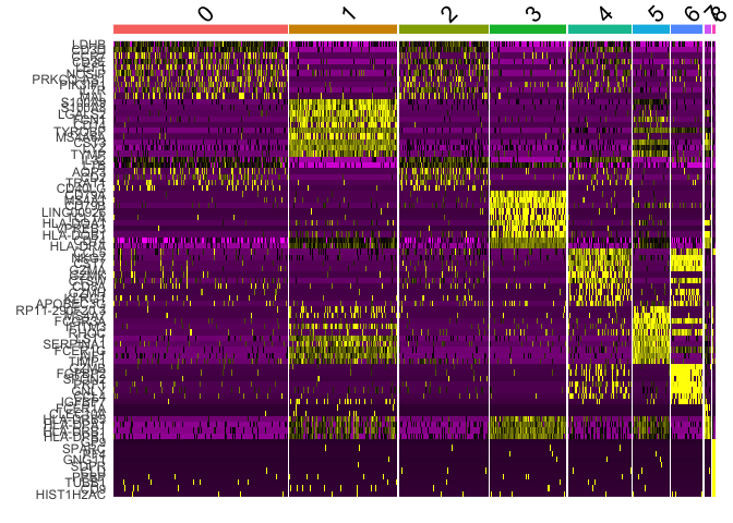
# Heatmap of top DEGs across clusters
pbmc_markers %>%
    group_by(cluster) %>%
    top_n(n = 10, wt = avg_log2FC) -> top10

pbmc_ser <- ScaleData(pbmc_ser,features=top10$gene)
## Centering and scaling data matrix
DoHeatmap(pbmc_ser, features = top10$gene) + NoLegend()
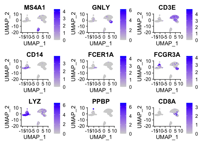
Identify cell types #
FeaturePlot(pbmc_ser, features = c("MS4A1", "GNLY", "CD3E", "CD14", "FCER1A", "FCGR3A", "LYZ", "PPBP","CD8A"))
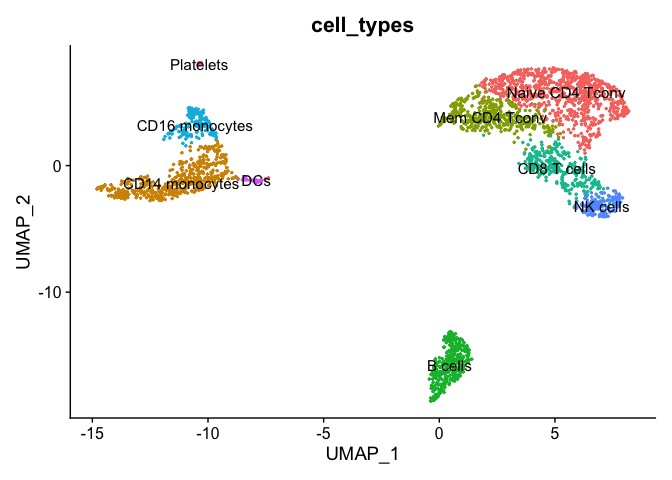
pbmc_meta <- pbmc_ser@meta.data %>%
    mutate(cell_types=RNA_snn_res.0.3) %>%
    mutate(cell_types=recode(cell_types,
        `0` = "Naive CD4 Tconv",
        `1` = "CD14 monocytes",
        `2` = "Mem CD4 Tconv",
        `3` = "B cells",
        `4` = "CD8 T cells",
        `5` = "CD16 monocytes",
        `6` = "NK cells",
        `7` = "DCs",
        `8` = "Platelets"
        )
    )

pbmc_meta %>%
    select(RNA_snn_res.0.3,cell_types) %>%
    table()
    ##                cell_types
    ## RNA_snn_res.0.3 Naive CD4 Tconv CD14 monocytes Mem CD4 Tconv B cells
    ##               0             781              0             0       0
    ##               1               0            483             0       0
    ##               2               0              0           399       0
    ##               3               0              0             0     344
    ##               4               0              0             0       0
    ##               5               0              0             0       0
    ##               6               0              0             0       0
    ##               7               0              0             0       0
    ##               8               0              0             0       0
    ##                cell_types
    ## RNA_snn_res.0.3 CD8 T cells CD16 monocytes NK cells DCs Platelets
    ##               0           0              0        0   0         0
    ##               1           0              0        0   0         0
    ##               2           0              0        0   0         0
    ##               3           0              0        0   0         0
    ##               4         283              0        0   0         0
    ##               5           0            162        0   0         0
    ##               6           0              0      143   0         0
    ##               7           0              0        0  29         0
    ##               8           0              0        0   0        14
pbmc_ser[["cell_types"]] <- pbmc_meta$cell_types

DimPlot(pbmc_ser, group.by="cell_types", reduction = "umap", label = TRUE, pt.size = 0.5) + NoLegend()
Shortcuts #
With the use of piping, we could have down much of this analysis in a few lines of code, as shown below.
pbmc_ser_quick <- CreateSeuratObject(counts=pbmc_data,project="pbmc3k",min.cells=3,min.features=200)
    ## Warning: Feature names cannot have underscores ('_'), replacing with dashes
    ## ('-')
pbmc_ser_quick[["percent_mt"]] <- PercentageFeatureSet(pbmc_ser_quick, pattern = "^MT-")

pbmc_ser_quick <- pbmc_ser_quick %>%
    subset(., subset = nFeature_RNA > 200 & nFeature_RNA < 2500 & percent_mt < 5) %>%
    NormalizeData(.) %>%
    FindVariableFeatures(.) %>%
    ScaleData(.) %>%
    RunPCA(.)
    ## Centering and scaling data matrix

    ## PC_ 1
    ## Positive:  CST3, TYROBP, LST1, AIF1, FTL, FTH1, LYZ, FCN1, S100A9, TYMP
    ##     FCER1G, CFD, LGALS1, S100A8, CTSS, LGALS2, SERPINA1, IFITM3, SPI1, CFP
    ##     PSAP, IFI30, SAT1, COTL1, S100A11, NPC2, GRN, LGALS3, GSTP1, PYCARD
    ## Negative:  MALAT1, LTB, IL32, IL7R, CD2, B2M, ACAP1, CD27, STK17A, CTSW
    ##     CD247, GIMAP5, AQP3, CCL5, SELL, TRAF3IP3, GZMA, MAL, CST7, ITM2A
    ##     MYC, GIMAP7, HOPX, BEX2, LDLRAP1, GZMK, ETS1, ZAP70, TNFAIP8, RIC3
    ## PC_ 2
    ## Positive:  CD79A, MS4A1, TCL1A, HLA-DQA1, HLA-DQB1, HLA-DRA, LINC00926, CD79B, HLA-DRB1, CD74
    ##     HLA-DMA, HLA-DPB1, HLA-DQA2, CD37, HLA-DRB5, HLA-DMB, HLA-DPA1, FCRLA, HVCN1, LTB
    ##     BLNK, P2RX5, IGLL5, IRF8, SWAP70, ARHGAP24, FCGR2B, SMIM14, PPP1R14A, C16orf74
    ## Negative:  NKG7, PRF1, CST7, GZMB, GZMA, FGFBP2, CTSW, GNLY, B2M, SPON2
    ##     CCL4, GZMH, FCGR3A, CCL5, CD247, XCL2, CLIC3, AKR1C3, SRGN, HOPX
    ##     TTC38, APMAP, CTSC, S100A4, IGFBP7, ANXA1, ID2, IL32, XCL1, RHOC
    ## PC_ 3
    ## Positive:  HLA-DQA1, CD79A, CD79B, HLA-DQB1, HLA-DPB1, HLA-DPA1, CD74, MS4A1, HLA-DRB1, HLA-DRA
    ##     HLA-DRB5, HLA-DQA2, TCL1A, LINC00926, HLA-DMB, HLA-DMA, CD37, HVCN1, FCRLA, IRF8
    ##     PLAC8, BLNK, MALAT1, SMIM14, PLD4, P2RX5, IGLL5, LAT2, SWAP70, FCGR2B
    ## Negative:  PPBP, PF4, SDPR, SPARC, GNG11, NRGN, GP9, RGS18, TUBB1, CLU
    ##     HIST1H2AC, AP001189.4, ITGA2B, CD9, TMEM40, PTCRA, CA2, ACRBP, MMD, TREML1
    ##     NGFRAP1, F13A1, SEPT5, RUFY1, TSC22D1, MPP1, CMTM5, RP11-367G6.3, MYL9, GP1BA
    ## PC_ 4
    ## Positive:  HLA-DQA1, CD79B, CD79A, MS4A1, HLA-DQB1, CD74, HIST1H2AC, HLA-DPB1, PF4, SDPR
    ##     TCL1A, HLA-DRB1, HLA-DPA1, HLA-DQA2, PPBP, HLA-DRA, LINC00926, GNG11, SPARC, HLA-DRB5
    ##     GP9, AP001189.4, CA2, PTCRA, CD9, NRGN, RGS18, CLU, TUBB1, GZMB
    ## Negative:  VIM, IL7R, S100A6, IL32, S100A8, S100A4, GIMAP7, S100A10, S100A9, MAL
    ##     AQP3, CD2, CD14, FYB, LGALS2, GIMAP4, ANXA1, CD27, FCN1, RBP7
    ##     LYZ, S100A11, GIMAP5, MS4A6A, S100A12, FOLR3, TRABD2A, AIF1, IL8, IFI6
    ## PC_ 5
    ## Positive:  GZMB, NKG7, S100A8, FGFBP2, GNLY, CCL4, CST7, PRF1, GZMA, SPON2
    ##     GZMH, S100A9, LGALS2, CCL3, CTSW, XCL2, CD14, CLIC3, S100A12, RBP7
    ##     CCL5, MS4A6A, GSTP1, FOLR3, IGFBP7, TYROBP, TTC38, AKR1C3, XCL1, HOPX
    ## Negative:  LTB, IL7R, CKB, VIM, MS4A7, AQP3, CYTIP, RP11-290F20.3, SIGLEC10, HMOX1
    ##     LILRB2, PTGES3, MAL, CD27, HN1, CD2, GDI2, CORO1B, ANXA5, TUBA1B
    ##     FAM110A, ATP1A1, TRADD, PPA1, CCDC109B, ABRACL, CTD-2006K23.1, WARS, VMO1, FYB
ElbowPlot(pbmc_ser_quick)

pbmc_ser_quick <- pbmc_ser_quick %>%
    RunUMAP(.,dims=1:7) %>%
    FindNeighbors(.,dims=1:7) %>%
    FindClusters(.,res=c(0.3,0.5,0.7))
## 22:21:16 UMAP embedding parameters a = 0.9922 b = 1.112
## 22:21:16 Read 2638 rows and found 7 numeric columns
## 22:21:16 Using Annoy for neighbor search, n_neighbors = 30
## 22:21:16 Building Annoy index with metric = cosine, n_trees = 50
## 0% 10 20 30 40 50 60 70 80 90 100%
## [----|----|----|----|----|----|----|----|----|----|
## **************************************************|
## 22:21:16 Writing NN index file to temp file /var/folders/1w/32zp8ffj6q50nny8nt6y1bvc0000gq/T//Rtmpfk3bAq/file75b85b03b68f
## 22:21:16 Searching Annoy index using 1 thread, search_k = 3000
## 22:21:17 Annoy recall = 100%
## 22:21:17 Commencing smooth kNN distance calibration using 1 thread with target n_neighbors = 30
## 22:21:17 Initializing from normalized Laplacian + noise (using irlba)
## 22:21:17 Commencing optimization for 500 epochs, with 102208 positive edges
## 22:21:19 Optimization finished
## Computing nearest neighbor graph
## Computing SNN
## Modularity Optimizer version 1.3.0 by Ludo Waltman and Nees Jan van Eck
##
## Number of nodes: 2638
## Number of edges: 88288
##
## Running Louvain algorithm...
## Maximum modularity in 10 random starts: 0.9150
## Number of communities: 9
## Elapsed time: 0 seconds
## Modularity Optimizer version 1.3.0 by Ludo Waltman and Nees Jan van Eck
##
## Number of nodes: 2638
## Number of edges: 88288
##
## Running Louvain algorithm...
## Maximum modularity in 10 random starts: 0.8827
## Number of communities: 10
## Elapsed time: 0 seconds
## Modularity Optimizer version 1.3.0 by Ludo Waltman and Nees Jan van Eck
##
## Number of nodes: 2638
## Number of edges: 88288
##
## Running Louvain algorithm...
## Maximum modularity in 10 random starts: 0.8576
## Number of communities: 11
## Elapsed time: 0 seconds
```tpl
Idents(pbmc_ser_quick) <- "RNA_snn_res.0.3"
DimPlot(pbmc_ser_quick,group.by="RNA_snn_res.0.3",label=T)

## Saving data
# saveRDS(pbmc_ser,file="pbmc3k_vignette_final_output_231024.rds")