Building more complex Seurat objects #

In most cases, we will want to go beyond reading one sample into Seurat and performing biological analyses. We often want to create a Seurat object that has multiple samples (e.g. biological replicates or patients). These samples will also have unique pieces of metadata, such as HPV- PBMC or HPV+ TIL from our head and neck cancer dataset.

Prerequisites #

This analysis assumes that you have download the samples described in the GEO download tutorial under utilities.

Load packages #

First, we will load the necessary packages.

library(Seurat)

    ## Attaching SeuratObject

library(dplyr)

    ##
    ## Attaching package: 'dplyr'

    ## The following objects are masked from 'package:stats':
    ## 
    ##     filter, lag

    ## The following objects are masked from 'package:base':
    ## 
    ##     intersect, setdiff, setequal, union

library(patchwork)

Read the individual files into a list #

The data I downloaded using the tutorial are located in /home/rstudio/docker_rstudio/data/geo_download. We will create a simple for loop to read all the files into individual variables stored in a list.

full_path <- "/home/rstudio/docker_rstudio/data/geo_download/"

raw_files <- list.files(paste(full_path))
# Not the metadata... we will use this in a second 
raw_files <- raw_files[2:5]
raw_files

    ## [1] "HD_PBMC_1" "HD_PBMC_2" "HD_PBMC_3" "HD_PBMC_4"

# Create list for Seurat object
raw_list <- vector("list",length=length(raw_files))
raw_list # empty list of length 4

    ## [[1]]
    ## NULL
    ## 
    ## [[2]]
    ## NULL
    ## 
    ## [[3]]
    ## NULL
    ## 
    ## [[4]]
    ## NULL

# Loop to read filtered feature barcode matrices into R data into R
for (i in 1:length(raw_list)) {
  
  raw_list[[i]] <- Read10X(paste(full_path,raw_files[i],sep=""))
  
}

dim(raw_list[[1]]) # 33694 genes by  2445 cells

    ## [1] 33694  2445

raw_list[[1]][1:50,1:10] # sparse matrix with counts

    ## 50 x 10 sparse Matrix of class "dgCMatrix"

    ##   [[ suppressing 10 column names 'AAACCTGCACAGACTT-1', 'AAACCTGCATCGGTTA-1', 'AAACCTGTCAAGCCTA-1' ... ]]

    ##                                  
    ## RP11-34P13.3  . . . . . . . . . .
    ## FAM138A       . . . . . . . . . .
    ## OR4F5         . . . . . . . . . .
    ## RP11-34P13.7  . . . . . . . . . .
    ## RP11-34P13.8  . . . . . . . . . .
    ## RP11-34P13.14 . . . . . . . . . .
    ## RP11-34P13.9  . . . . . . . . . .
    ## FO538757.3    . . . . . . . . . .
    ## FO538757.2    . . . . . . 1 . . .
    ## AP006222.2    1 . . . . . . . . .
    ## RP5-857K21.15 . . . . . . . . . .
    ## RP4-669L17.2  . . . . . . . . . .
    ## RP4-669L17.10 . . . . . . . . . .
    ## OR4F29        . . . . . . . . . .
    ## RP5-857K21.4  . . . . . . . . . .
    ## RP5-857K21.2  . . . . . . . . . .
    ## OR4F16        . . . . . . . . . .
    ## RP11-206L10.4 . . . . . . . . . .
    ## RP11-206L10.9 . . . . . . . . . .
    ## FAM87B        . . . . . . . . . .
    ## LINC00115     . . . . . . . . . .
    ## FAM41C        . . . . . . . . . .
    ## RP11-54O7.16  . . . . . . . . . .
    ## RP11-54O7.1   . . . . . . . . . .
    ## RP11-54O7.2   . . . . . . . . . .
    ## RP11-54O7.3   . . . . . . . . . .
    ## SAMD11        . . . . . . . . . .
    ## NOC2L         . . . 2 . . . . . .
    ## KLHL17        . . . . . . . . . .
    ## PLEKHN1       . . . . . . . . . .
    ## PERM1         . . . . . . . . . .
    ## RP11-54O7.17  . . . . . . . . . .
    ## HES4          . . . . . . . . . .
    ## ISG15         . 4 1 . . . 1 1 . .
    ## RP11-54O7.11  . . . . . . . . . .
    ## AGRN          . . . . . . . . . .
    ## RP11-54O7.18  . . . . . . . . . .
    ## RNF223        . . . . . . . . . .
    ## C1orf159      . . . . . . . . . .
    ## LINC01342     . . . . . . . . . .
    ## RP11-465B22.8 . . . . . . . . . .
    ## TTLL10-AS1    . . . . . . . . . .
    ## TTLL10        . . . . . . . . . .
    ## TNFRSF18      . . . . . . . . . .
    ## TNFRSF4       . . . 1 1 . . 1 . .
    ## SDF4          . . . . . . . 1 . .
    ## B3GALT6       . . . . . . . . . .
    ## FAM132A       . . . . . . . . . .
    ## RP5-902P8.12  . . . . . . . . . .
    ## UBE2J2        . . . . . . . . . .

# Name each item in the list by its title
names(raw_list) <- raw_files
names(raw_list)

    ## [1] "HD_PBMC_1" "HD_PBMC_2" "HD_PBMC_3" "HD_PBMC_4"

Read in metadata #

Before we construct the combined object, we will need the metadata.

We can read that in from the tsv file using readr::read_tsv (readr is a package, and the “::” lets us call a function from that package without loading the package)

# Read in the metadata
metadata_file <- readr::read_tsv("/home/rstudio/docker_rstudio/data/geo_download/GSE139324_metadata.tsv")

    ## Rows: 63 Columns: 45
    ## ── Column specification ────────────────────────────────────────────────────────
    ## Delimiter: "\t"
    ## chr (41): sample_accession, title, geo_accession, status, submission_date, l...
    ## dbl  (4): channel_count, taxid_ch1, contact_zip/postal_code, data_row_count
    ## 
    ## ℹ Use `spec()` to retrieve the full column specification for this data.
    ## ℹ Specify the column types or set `show_col_types = FALSE` to quiet this message.

# Re-name a few columns for easy use 
colnames(metadata_file)[c(43,45)] <- c("disease_state","tissue")

# Filter to only our samples of interest
metadata_file_filtered <- metadata_file %>%
  filter(title %in% raw_files)

# Make sure the order of names matches the raw data list 
identical(metadata_file_filtered$title,names(raw_list))

    ## [1] TRUE

# Create an empty list of Seurat objects
ser_list <- vector("list",length=length(raw_list))

# Loop to Create individual Seurat objects and include metadata 
for (i in 1:length(ser_list)) {
  
  # Create Seurat Object
  ser_list[[i]] <- CreateSeuratObject(raw_list[[i]])
  
  # Create metadata for each object
  meta_add <- data.frame(matrix(data=NA,nrow=ncol(ser_list[[i]]),ncol=3))
  colnames(meta_add) <- c("title","disease_state","tissue")
  rownames(meta_add) <- colnames(ser_list[[i]])
  meta_add$title <- metadata_file_filtered[i,"title"] %>% pull()
  meta_add$disease_state <- metadata_file_filtered[i,"disease_state"] %>% pull()
  meta_add$tissue <- metadata_file_filtered[i,"tissue"] %>% pull()
  
  # Add Metadata
  ser_list[[i]] <- AddMetaData(ser_list[[i]],metadata=meta_add)

}

    ## Warning: Feature names cannot have underscores ('_'), replacing with dashes
    ## ('-')

    ## Warning: Feature names cannot have underscores ('_'), replacing with dashes
    ## ('-')

    ## Warning: Feature names cannot have underscores ('_'), replacing with dashes
    ## ('-')

    ## Warning: Feature names cannot have underscores ('_'), replacing with dashes
    ## ('-')

# Check out our list of Seurat objects
ser_list

    ## [[1]]
    ## An object of class Seurat 
    ## 33694 features across 2445 samples within 1 assay 
    ## Active assay: RNA (33694 features, 0 variable features)
    ## 
    ## [[2]]
    ## An object of class Seurat 
    ## 33694 features across 2436 samples within 1 assay 
    ## Active assay: RNA (33694 features, 0 variable features)
    ## 
    ## [[3]]
    ## An object of class Seurat 
    ## 33694 features across 1767 samples within 1 assay 
    ## Active assay: RNA (33694 features, 0 variable features)
    ## 
    ## [[4]]
    ## An object of class Seurat 
    ## 33694 features across 2315 samples within 1 assay 
    ## Active assay: RNA (33694 features, 0 variable features)

Merge list of Seurat objects into a single seurat object #

ser_merged <- merge(ser_list[[1]],ser_list[2:4])

    ## Warning in CheckDuplicateCellNames(object.list = objects): Some cell names are
    ## duplicated across objects provided. Renaming to enforce unique cell names.

ser_merged@meta.data$title %>%
  table()

    ## .
    ## HD_PBMC_1 HD_PBMC_2 HD_PBMC_3 HD_PBMC_4 
    ##      2445      2436      1767      2315

ser_merged@meta.data %>%
  select(title,disease_state) %>%
  table()

    ##            disease_state
    ## title       Healthy donor
    ##   HD_PBMC_1          2445
    ##   HD_PBMC_2          2436
    ##   HD_PBMC_3          1767
    ##   HD_PBMC_4          2315

ser_merged@meta.data %>%
  select(title,tissue) %>%
  table()

    ##            tissue
    ## title       peripheral blood
    ##   HD_PBMC_1             2445
    ##   HD_PBMC_2             2436
    ##   HD_PBMC_3             1767
    ##   HD_PBMC_4             2315

Analysis of all 4 samples #

As per the shortcut in the PBMC vignette, here’s a quick analysis of the 4 healthy donor samples we merged into one Seurat object.

ser_merged <- ser_merged %>%
  NormalizeData() %>%
  FindVariableFeatures() %>%
  ScaleData() %>%
  RunPCA()

    ## Centering and scaling data matrix

    ## PC_ 1 
    ## Positive:  RPS29, IL32, TRAC, LTB, RPS18, TRBC2, IL7R, RPS12, TRBC1, RPS2 
    ##     EEF1A1, CCR7, CD247, CD69, PEBP1, TRAT1, GZMM, MYC, AQP3, TSHZ2 
    ##     CTSW, FHIT, NGFRAP1, CDC25B, RPS26, HIST1H4C, FKBP11, NELL2, CD8B, CD40LG 
    ## Negative:  CST3, FCN1, LYZ, CSTA, LST1, S100A9, CTSS, TYROBP, S100A8, MNDA 
    ##     FGL2, FTL, SAT1, TYMP, FTH1, VCAN, PSAP, FOS, LGALS1, FCER1G 
    ##     S100A12, SERPINA1, CFD, CYBB, NEAT1, SPI1, MS4A6A, AIF1, HLA-DRA, GPX1 
    ## PC_ 2 
    ## Positive:  LTB, CCR7, RPS12, RPS18, EEF1A1, RPS2, RPLP1, CD79A, MYC, MS4A1 
    ##     IGHM, IL7R, NCF1, IGHD, LINC00926, BANK1, BIRC3, VPREB3, RPS29, FHIT 
    ##     TSHZ2, TCL1A, VIM, CD22, IGKC, TNFRSF13C, NGFRAP1, TRAC, FCRLA, FCER2 
    ## Negative:  NKG7, CST7, GZMA, PRF1, GNLY, KLRD1, GZMB, FGFBP2, HOPX, CTSW 
    ##     KLRF1, CCL5, SPON2, GZMH, TRDC, FCGR3A, CLIC3, CCL4, MATK, KLRB1 
    ##     ADGRG1, MYO1F, PFN1, S1PR5, C12orf75, CMC1, IL2RB, TTC38, PRSS23, C1orf21 
    ## PC_ 3 
    ## Positive:  TRAC, IL7R, IL32, VIM, S100A6, S100A12, VCAN, S100A8, ANXA1, S100A9 
    ##     CXCL8, TRAT1, S100A4, TRBC1, MCL1, CD14, CH17-373J23.1, RGCC, LYZ, IL1B 
    ##     AIF1, NEAT1, FHIT, RBP7, NFKBIZ, RP11-160E2.6, TSHZ2, CSTA, DUSP6, TSPO 
    ## Negative:  CD79A, MS4A1, IGHM, CD79B, IGKC, LINC00926, IGHD, BANK1, TCL1A, VPREB3 
    ##     SPIB, HLA-DQA1, CD22, FAM129C, BLNK, HLA-DPA1, CD74, FCRLA, HLA-DPB1, FCER2 
    ##     TSPAN13, HLA-DOB, HLA-DQB1, TNFRSF13C, IGLC2, BLK, JCHAIN, CD19, CD24, RP11-693J15.5 
    ## PC_ 4 
    ## Positive:  CDKN1C, HES4, CKB, CSF1R, TCF7L2, MS4A4A, SIGLEC10, CTD-2006K23.1, HMOX1, FCGR3A 
    ##     MS4A7, VMO1, BATF3, LINC01272, LRRC25, ZNF703, IFITM3, FAM110A, LYPD2, ICAM4 
    ##     CTSL, CDH23, TPPP3, RHOC, C1QA, LILRB2, PILRA, BID, OAS1, CD68 
    ## Negative:  CXCL8, VCAN, S100A12, IL1B, RP11-160E2.6, CH17-373J23.1, NFKBIA, FOSB, CCL3, FOS 
    ##     S100A8, IER3, CTD-3252C9.4, TNFAIP3, JUN, RP11-1143G9.4, EGR1, NCF1, JUND, LUCAT1 
    ##     S100A9, ITGAM, CD14, LINC00936, MT-CO1, MCL1, MS4A6A, KLF10, CYP1B1, CLEC4E 
    ## PC_ 5 
    ## Positive:  CD79B, MS4A1, CD79A, LINC00926, IGHD, FCGR3A, CDKN1C, VPREB3, CD22, FCER2 
    ##     BANK1, MS4A7, SIGLEC10, IGHM, HES4, FCRL1, TNFRSF13C, CKB, MTSS1, TCF7L2 
    ##     LINC01272, HLA-DOB, FCRLA, RP11-693J15.5, CD19, CD24, RALGPS2, CD72, SWAP70, HMOX1 
    ## Negative:  SERPINF1, PLD4, GAS6, LRRC26, PPP1R14B, CLEC4C, LILRA4, ITM2C, TPM2, FCER1A 
    ##     DERL3, SCT, PTCRA, SMPD3, C1orf186, JCHAIN, LINC00996, SCN9A, IL3RA, LILRB4 
    ##     PTPRS, CCDC50, RP11-117D22.2, MZB1, UGCG, RP11-73G16.2, DNASE1L3, LAMP5, MAP1A, TNFRSF21

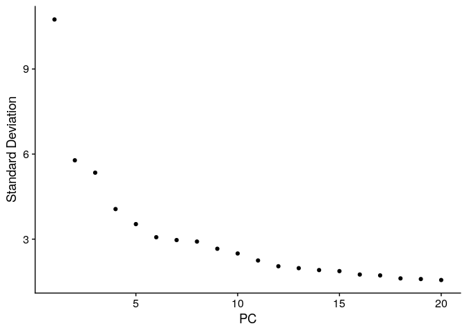
ElbowPlot(ser_merged)

ser_merged <- ser_merged %>%
  FindNeighbors(.,dims=1:15) %>%
  FindClusters(.,res=c(0.3,0.5,0.7)) %>% 
  RunUMAP(.,dims=1:10)

    ## Computing nearest neighbor graph

    ## Computing SNN

    ## Modularity Optimizer version 1.3.0 by Ludo Waltman and Nees Jan van Eck
    ## 
    ## Number of nodes: 8963
    ## Number of edges: 319663
    ## 
    ## Running Louvain algorithm...
    ## Maximum modularity in 10 random starts: 0.9303
    ## Number of communities: 13
    ## Elapsed time: 0 seconds
    ## Modularity Optimizer version 1.3.0 by Ludo Waltman and Nees Jan van Eck
    ## 
    ## Number of nodes: 8963
    ## Number of edges: 319663
    ## 
    ## Running Louvain algorithm...
    ## Maximum modularity in 10 random starts: 0.9083
    ## Number of communities: 16
    ## Elapsed time: 0 seconds
    ## Modularity Optimizer version 1.3.0 by Ludo Waltman and Nees Jan van Eck
    ## 
    ## Number of nodes: 8963
    ## Number of edges: 319663
    ## 
    ## Running Louvain algorithm...
    ## Maximum modularity in 10 random starts: 0.8883
    ## Number of communities: 17
    ## Elapsed time: 0 seconds

    ## Warning: The default method for RunUMAP has changed from calling Python UMAP via reticulate to the R-native UWOT using the cosine metric
    ## To use Python UMAP via reticulate, set umap.method to 'umap-learn' and metric to 'correlation'
    ## This message will be shown once per session

    ## 19:09:30 UMAP embedding parameters a = 0.9922 b = 1.112

    ## 19:09:30 Read 8963 rows and found 10 numeric columns

    ## 19:09:30 Using Annoy for neighbor search, n_neighbors = 30

    ## 19:09:30 Building Annoy index with metric = cosine, n_trees = 50

    ## 0%   10   20   30   40   50   60   70   80   90   100%

    ## [----|----|----|----|----|----|----|----|----|----|

    ## **************************************************|
    ## 19:09:30 Writing NN index file to temp file /tmp/RtmpZYOKxd/file44aa2cf3936a
    ## 19:09:30 Searching Annoy index using 1 thread, search_k = 3000
    ## 19:09:32 Annoy recall = 100%
    ## 19:09:32 Commencing smooth kNN distance calibration using 1 thread with target n_neighbors = 30
    ## 19:09:33 Initializing from normalized Laplacian + noise (using irlba)
    ## 19:09:33 Commencing optimization for 500 epochs, with 368458 positive edges
    ## 19:09:38 Optimization finished

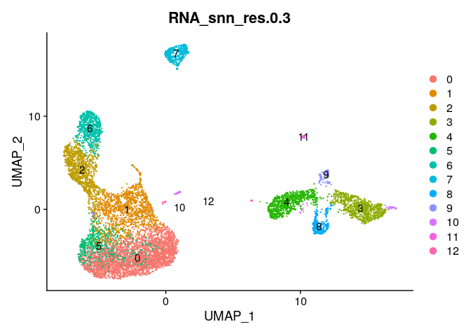
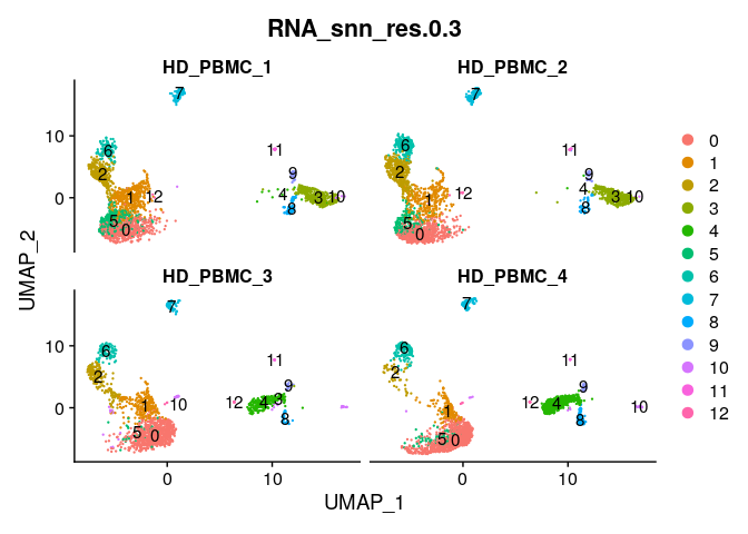
Plot a UMAP of clusters by sample #

DimPlot(ser_merged,group.by="RNA_snn_res.0.3",label=T)

DimPlot(ser_merged,group.by="RNA_snn_res.0.3",split.by="title",label=T,
        ncol=2)

Save output #

save_path <- "/home/rstudio/docker_rstudio/data/"
saveRDS(ser_merged,file=paste(save_path,"ser_merged_4_hd_pbmc_231027.rds",sep=""))