Intro to data integration #
A recurrent theme in -omics work is the notion of “batch effects”. This term originates from the days of microarrays, when there would be slight differences in annealing times and/or affinities between runs of microarrays. “Batch effects” has now become a blanket colloquial term to generally mean anything related to a technical artifact that arises between samples or runs. The key is that it is not a true biological signal, but instead something that should be “normalized away” to allow real biological signals to shine.
Statistically, it is straightforward to control for a batch effect: if you are using a linear model, for example, you could include the “batch” as a covariate. The challenge really arises with high-dimensional approaches such as principal component analysis or visualizing data in a UMAP - often times, when batch effects are present, visualizations are distorted or largely driven by these batch effects. There are well-documented strategies for removing batch effect in microarrays or bulk RNAseq data, which we will not discuss here.
For single-cell RNAseq analysis, we can use one simple approach called “data integration” that is robustly implemented in Seurat. To demonstrate this, we will use healthy donor PBMC that have been generated with either 10X Genomics 3’ v2 chemistry or 5’ v1 chemistry. The chemistry, in this case, is the batch effect we are trying to remove.
Prerequisites #
We will need to download some dataset from the Cillo Laboratory tutorial_datasets github page.
If you navigate to the link, click the code button on the top right, and click “Download ZIP” it will download the whole repository including directories containing the 10X scRNAseq datasets.
For this tutorial, we will be using the PBMC_integration_datasets directory and enclosed files.
Load packages #
library(Seurat)
## Attaching SeuratObject
library(dplyr)
    ##
    ## Attaching package: 'dplyr'

    ## The following objects are masked from 'package:stats':
    ##
    ##     filter, lag

    ## The following objects are masked from 'package:base':
    ##
    ##     intersect, setdiff, setequal, union
library(patchwork)

full_path <- "/home/rstudio/docker_rstudio/data/tutorial_datasets-main/PBMC_integration_datasets/"

raw_files <- list.files(paste(full_path))

# We don't want to read in the metadata as a 10X dataset
# Let's remove it from the raw_files
raw_files <- raw_files[!grepl("txt",raw_files)]
raw_files
## [1] "HD_PBMC_1" "HD_PBMC_1_5prime" "HD_PBMC_2" "HD_PBMC_2_5prime"
# Create list for Seurat object
raw_list <- vector("list",length=length(raw_files))
raw_list # empty list of length 4
    ## [[1]]
    ## NULL
    ##
    ## [[2]]
    ## NULL
    ##
    ## [[3]]
    ## NULL
    ##
    ## [[4]]
    ## NULL
# Loop to read filtered feature barcode matrices into R data into R
for (i in 1:length(raw_list)) {

  raw_list[[i]] <- Read10X(paste(full_path,raw_files[i],sep=""))

}

# Name each item in the list by its title
names(raw_list) <- raw_files
names(raw_list)
## [1] "HD_PBMC_1" "HD_PBMC_1_5prime" "HD_PBMC_2" "HD_PBMC_2_5prime"
Read in metadata and create Seurat objects #
# Read in the metadata
metadata_file <- readr::read_tsv(paste(full_path,"pbmc_integration_metadata.txt",
                                       sep=""))
    ## Rows: 4 Columns: 3
    ## ── Column specification ────────────────────────────────────────────────────────
    ## Delimiter: "\t"
    ## chr (3): sample_id, sample_type, chemistry
    ##
    ## ℹ Use `spec()` to retrieve the full column specification for this data.
    ## ℹ Specify the column types or set `show_col_types = FALSE` to quiet this message.
# Make sure the order of names matches the raw data list
identical(metadata_file$sample_id,names(raw_list))
## [1] TRUE
# Create an empty list of Seurat objects
ser_list <- vector("list",length=length(raw_list))

# Loop to Create individual Seurat objects and include metadata
for (i in 1:length(ser_list)) {

  # Create Seurat Object
  ser_list[[i]] <- CreateSeuratObject(raw_list[[i]])

  # Create metadata for each object
  meta_add <- data.frame(matrix(data=NA,
                                nrow=ncol(ser_list[[i]]),
                                ncol=ncol(metadata_file))
                         )
  colnames(meta_add) <- colnames(metadata_file)
  rownames(meta_add) <- colnames(ser_list[[i]])
  meta_add[,1] <- metadata_file[i,1] %>% pull()
  meta_add[,2] <- metadata_file[i,2] %>% pull()
  meta_add[,3] <- metadata_file[i,3] %>% pull()

  # Add Metadata
  ser_list[[i]] <- AddMetaData(ser_list[[i]],metadata=meta_add)

}
    ## Warning: Feature names cannot have underscores ('_'), replacing with dashes
    ## ('-')

    ## Warning: Feature names cannot have underscores ('_'), replacing with dashes
    ## ('-')

    ## Warning: Feature names cannot have underscores ('_'), replacing with dashes
    ## ('-')

    ## Warning: Feature names cannot have underscores ('_'), replacing with dashes
    ## ('-')
# Check out our list of Seurat objects
ser_list
    ## [[1]]
    ## An object of class Seurat
    ## 33694 features across 2445 samples within 1 assay
    ## Active assay: RNA (33694 features, 0 variable features)
    ##
    ## [[2]]
    ## An object of class Seurat
    ## 33694 features across 1451 samples within 1 assay
    ## Active assay: RNA (33694 features, 0 variable features)
    ##
    ## [[3]]
    ## An object of class Seurat
    ## 33694 features across 2436 samples within 1 assay
    ## Active assay: RNA (33694 features, 0 variable features)
    ##
    ## [[4]]
    ## An object of class Seurat
    ## 33694 features across 1501 samples within 1 assay
    ## Active assay: RNA (33694 features, 0 variable features)
Merge list of Seurat objects into a single seurat object #
ser_merged <- merge(ser_list[[1]],ser_list[2:length(ser_list)])
    ## Warning in CheckDuplicateCellNames(object.list = objects): Some cell names are
    ## duplicated across objects provided. Renaming to enforce unique cell names.
ser_merged@meta.data$sample_id %>%
  table()
    ## .
    ##        HD_PBMC_1 HD_PBMC_1_5prime        HD_PBMC_2 HD_PBMC_2_5prime
    ##             2445             1451             2436             1501
ser_merged@meta.data %>%
  select(sample_id,chemistry) %>%
  table()
    ##                   chemistry
    ## sample_id          3prime 5prime
    ##   HD_PBMC_1          2445      0
    ##   HD_PBMC_1_5prime      0   1451
    ##   HD_PBMC_2          2436      0
    ##   HD_PBMC_2_5prime      0   1501
QC filtering #
Now that we have out combined object, let’s perform some filtering before we integrate.
ser_merged[["percent_mt"]] <- PercentageFeatureSet(ser_merged, pattern = "^MT-")

# Check out metadata now
head(ser_merged@meta.data)
    ##                         orig.ident nCount_RNA nFeature_RNA sample_id
    ## AAACCTGCACAGACTT-1_1 SeuratProject       5192         1151 HD_PBMC_1
    ## AAACCTGCATCGGTTA-1_1 SeuratProject       2368          986 HD_PBMC_1
    ## AAACCTGTCAAGCCTA-1_1 SeuratProject       6676         1419 HD_PBMC_1
    ## AAACCTGTCTTAACCT-1_1 SeuratProject       2898         1050 HD_PBMC_1
    ## AAACGGGCAATAGCGG-1_1 SeuratProject       5450         1187 HD_PBMC_1
    ## AAACGGGGTAGCGATG-1_1 SeuratProject      11649         2338 HD_PBMC_1
    ##                      sample_type chemistry percent_mt
    ## AAACCTGCACAGACTT-1_1        PBMC    3prime   4.160247
    ## AAACCTGCATCGGTTA-1_1        PBMC    3prime   9.459459
    ## AAACCTGTCAAGCCTA-1_1        PBMC    3prime   4.988017
    ## AAACCTGTCTTAACCT-1_1        PBMC    3prime   5.279503
    ## AAACGGGCAATAGCGG-1_1        PBMC    3prime   4.623853
    ## AAACGGGGTAGCGATG-1_1        PBMC    3prime   3.802902
# We can also plot values from metadata
VlnPlot(ser_merged, features = c("nFeature_RNA", "nCount_RNA", "percent_mt"), ncol = 3)
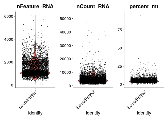
# Filtering is often dataset specific
# Here, we want more than 200 and less than 3000 features
# Plus % mito < 20%
ser_merged <- subset(ser_merged, subset = nFeature_RNA > 200 & nFeature_RNA < 3000 & percent_mt < 20)

# Check out the cells left
ser_merged@meta.data %>%
  select(sample_id,chemistry) %>%
  table()
    ##                   chemistry
    ## sample_id          3prime 5prime
    ##   HD_PBMC_1          2436      0
    ##   HD_PBMC_1_5prime      0   1284
    ##   HD_PBMC_2          2428      0
    ##   HD_PBMC_2_5prime      0   1380
Standard workflow #
We will run the standard workflow first to demonstrate the chemistry specific batch effects.
# Store the filtered and un-manipulated dataset
ser_merged_save <- ser_merged

ser_merged <- ser_merged %>%
    NormalizeData(.) %>%
    FindVariableFeatures(.) %>%
    ScaleData(.) %>%
    RunPCA(.)
    ## Centering and scaling data matrix

    ## PC_ 1
    ## Positive:  IL32, CD3E, RPS18, RPS12, RPL30, EEF1A1, LTB, LDHB, RPS21, TRBC2
    ##     IFITM1, TRAC, IL7R, CD7, RPLP0, RPS8, RPL37, TRBC1, TCF7, NOSIP
    ##     LINC00861, CD69, CCR7, GZMM, LEF1, CAMK4, MAL, CD247, FLT3LG, FCMR
    ## Negative:  FCN1, CST3, LYZ, S100A9, S100A8, VCAN, MNDA, FGL2, CTSS, LST1
    ##     SERPINA1, CYBB, CD14, CSTA, MS4A6A, MPEG1, SAT1, CLEC7A, TYMP, TYROBP
    ##     SPI1, S100A12, FTL, PSAP, FOS, CSF3R, NCF2, TMEM176B, GRN, NEAT1
    ## PC_ 2
    ## Positive:  RPS17, LTB, RPS18, RPLP1, RPS8, RPS12, CCR7, EEF1A1, LDHB, TPT1
    ##     MAL, CD79A, LEF1, RPL30, RPLP0, RPL37, TRABD2A, TCF7, MS4A1, TRAC
    ##     NOSIP, LINC00926, FHIT, MYC, HLA-DRA, BANK1, BIRC3, SELL, AIF1, NCF1
    ## Negative:  CST7, NKG7, PRF1, GZMA, GNLY, KLRD1, GZMB, CTSW, FGFBP2, CCL5
    ##     HOPX, SPON2, GZMH, ADGRG1, HLA-B, FCGR3A, KLRF1, CCL4, S1PR5, IL2RB
    ##     HLA-C, MATK, CD247, CD99, PFN1, CLIC3, HLA-A, ITGB2, PRSS23, IFITM2
    ## PC_ 3
    ## Positive:  TMSB4X, S100A6, TRAC, RPS17, CXCL8, IL1B, S100A4, TNFAIP3, S100A9, NEAT1
    ##     S100A12, S100A8, IL32, NAMPT, NFKBIA, CSTA, NFKBIZ, ANXA1, CH17-373J23.1, CCL3
    ##     AIF1, LDHB, FOS, CD3E, IER3, LYZ, VCAN, NOSIP, SRGN, CTD-3252C9.4
    ## Negative:  MS4A1, CD79A, BANK1, FAM129C, LINC00926, CD19, CD79B, TCL1A, FCRLA, HLA-DQA1
    ##     FCER2, VPREB3, IGHM, HLA-DOB, BLNK, BLK, CD22, RALGPS2, IGHD, FCRL1
    ##     IGKC, RP11-693J15.5, CD74, SPIB, HLA-DQA2, POU2AF1, PAX5, TSPAN13, HLA-DPA1, HVCN1
    ## PC_ 4
    ## Positive:  MT-ATP8, MTRNR2L12, MT-ND4L, AC090498.1, EEF1G, COL6A3, GABARAP, NME2, GIMAP7, PTPRCAP
    ##     IL7R, MT-ATP6, ATP6V0C, RPS21, MT-ND6, GIMAP4, LIME1, RP11-290D2.6, TPT1, CD3E
    ##     DGKA, HIST1H4C, LEF1, RPL37, CTB-133G6.1, CCR7, INPP4B, AC006129.2, RPL30, MT-ND5
    ## Negative:  RPS17, TMSB4X, NFKBIA, CYBA, GNLY, NKG7, GZMB, KLRF1, TRDC, IL1B
    ##     CCL4, FGFBP2, HOPX, SPON2, CXCL8, C1orf56, ID2, KLRD1, NR4A2, GZMA
    ##     CCL3, DUSP1, CLIC3, CCL5, FCGR3A, FCER1G, CST7, TYROBP, GZMH, KLRB1
    ## PC_ 5
    ## Positive:  CXCL8, IL1B, CH17-373J23.1, RP11-1143G9.4, RP11-160E2.6, S100A12, CCL3, FOSB, IER3, MT-ATP6
    ##     MCL1, LINC00936, MT-CO2, NAMPT, LUCAT1, CTB-61M7.2, PTPRCAP, KLF6, CTDSPL, TMEM107
    ##     PTGS2, NFKBIA, KLF10, S100A8, CCL3L3, VCAN, ANKRD28, TRIB1, TNFAIP3, ZFP36L1
    ## Negative:  LILRA4, CDKN1C, PLD4, CSF1R, SERPINF1, CKB, IL3RA, LILRB4, HES4, LILRB2
    ##     LILRB1, PPP1R14B, CD68, TBC1D8, GAS6, LRRC26, PTCRA, CLEC4C, TCF7L2, SMPD3
    ##     MS4A4A, HMOX1, FCGR3A, RHOC, LINC00996, SCT, LRRC25, CDH23, SIGLEC10, TPM2
ElbowPlot(ser_merged)
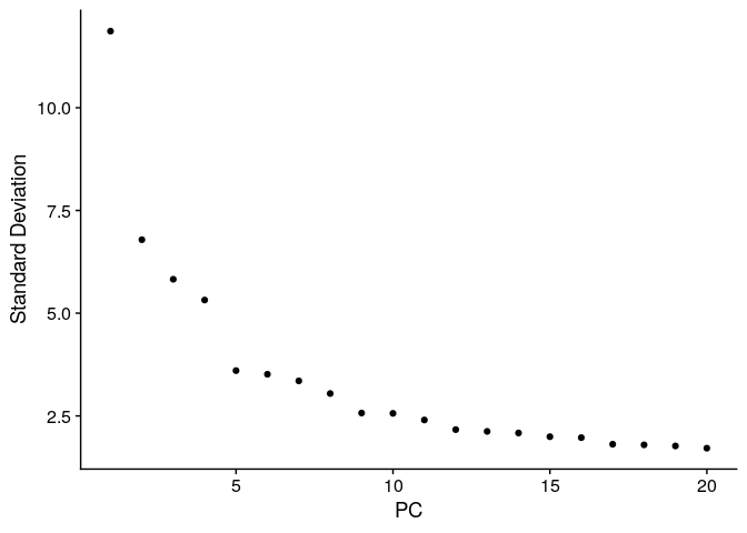
ser_merged <- ser_merged %>%
    RunUMAP(.,dims=1:10) %>%
    FindNeighbors(.,dims=1:10) %>%
    FindClusters(.,res=c(0.3,0.5,0.7))
    ## Warning: The default method for RunUMAP has changed from calling Python UMAP via reticulate to the R-native UWOT using the cosine metric
    ## To use Python UMAP via reticulate, set umap.method to 'umap-learn' and metric to 'correlation'
    ## This message will be shown once per session

    ## 21:14:16 UMAP embedding parameters a = 0.9922 b = 1.112

    ## 21:14:16 Read 7528 rows and found 10 numeric columns

    ## 21:14:16 Using Annoy for neighbor search, n_neighbors = 30

    ## 21:14:16 Building Annoy index with metric = cosine, n_trees = 50

    ## 0%   10   20   30   40   50   60   70   80   90   100%

    ## [----|----|----|----|----|----|----|----|----|----|

    ## **************************************************|
    ## 21:14:16 Writing NN index file to temp file /tmp/Rtmp1pnHMW/file1b6541c7897
    ## 21:14:16 Searching Annoy index using 1 thread, search_k = 3000
    ## 21:14:18 Annoy recall = 100%
    ## 21:14:18 Commencing smooth kNN distance calibration using 1 thread with target n_neighbors = 30
    ## 21:14:18 Initializing from normalized Laplacian + noise (using irlba)
    ## 21:14:18 Commencing optimization for 500 epochs, with 311174 positive edges
    ## 21:14:23 Optimization finished
    ## Computing nearest neighbor graph
    ## Computing SNN

    ## Modularity Optimizer version 1.3.0 by Ludo Waltman and Nees Jan van Eck
    ##
    ## Number of nodes: 7528
    ## Number of edges: 263376
    ##
    ## Running Louvain algorithm...
    ## Maximum modularity in 10 random starts: 0.9513
    ## Number of communities: 14
    ## Elapsed time: 0 seconds
    ## Modularity Optimizer version 1.3.0 by Ludo Waltman and Nees Jan van Eck
    ##
    ## Number of nodes: 7528
    ## Number of edges: 263376
    ##
    ## Running Louvain algorithm...
    ## Maximum modularity in 10 random starts: 0.9319
    ## Number of communities: 15
    ## Elapsed time: 0 seconds
    ## Modularity Optimizer version 1.3.0 by Ludo Waltman and Nees Jan van Eck
    ##
    ## Number of nodes: 7528
    ## Number of edges: 263376
    ##
    ## Running Louvain algorithm...
    ## Maximum modularity in 10 random starts: 0.9125
    ## Number of communities: 15
    ## Elapsed time: 0 seconds
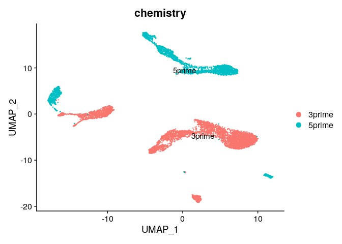
Idents(ser_merged) <- "RNA_snn_res.0.3"

DimPlot(ser_merged,group.by="chemistry",label=T)
DimPlot(ser_merged,group.by="RNA_snn_res.0.3",split.by="chemistry",label=T)
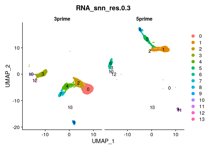
# Check out chemistry-specific clusters
ser_merged@meta.data %>%
  select(RNA_snn_res.0.3,chemistry) %>%
  table()
    ##                chemistry
    ## RNA_snn_res.0.3 3prime 5prime
    ##              0    1748      2
    ##              1       0   1216
    ##              2     818      6
    ##              3     767      3
    ##              4     700      0
    ##              5       0    564
    ##              6       0    458
    ##              7     398      0
    ##              8       0    254
    ##              9     212      4
    ##              10    127     20
    ##              11      0    130
    ##              12     61      2
    ##              13     33      5
Batch effects #
Clearly, there are strong batch effects associated with the chemistry used to generated the data. Let’s look at how we can correct these batch effects by integrating the datasets.
We will use the SCTransform and rpca approaches described by the Satija Lab in Seurat. More info on integration approaches is available here.
ser_merged_split <- SplitObject(ser_merged, split.by = "chemistry")

# lapply applies the FUN (function) to each member of the list and returns a list
ser_merged_split <- lapply(X = ser_merged_split, FUN = SCTransform, method = "glmGamPoi")
## Calculating cell attributes from input UMI matrix: log_umi
## Variance stabilizing transformation of count matrix of size 15205 by 4864
## Model formula is y ~ log_umi
## Get Negative Binomial regression parameters per gene
## Using 2000 genes, 4864 cells
## | | | 0% | |================== | 25% | |=================================== | 50% | |==================================================== | 75% | |======================================================================| 100%
## Found 102 outliers - those will be ignored in fitting/regularization step
## Second step: Get residuals using fitted parameters for 15205 genes
## | | | 0% | |== | 3% | |===== | 6% | |======= | 10% | |========= | 13% | |=========== | 16% | |============== | 19% | |================ | 23% | |================== | 26% | |==================== | 29% | |======================= | 32% | |========================= | 35% | |=========================== | 39% | |============================= | 42% | |================================ | 45% | |================================== | 48% | |==================================== | 52% | |====================================== | 55% | |========================================= | 58% | |=========================================== | 61% | |============================================= | 65% | |=============================================== | 68% | |================================================== | 71% | |==================================================== | 74% | |====================================================== | 77% | |======================================================== | 81% | |=========================================================== | 84% | |============================================================= | 87% | |=============================================================== | 90% | |================================================================= | 94% | |==================================================================== | 97% | |======================================================================| 100%
## Computing corrected count matrix for 15205 genes
## | | | 0% | |== | 3% | |===== | 6% | |======= | 10% | |========= | 13% | |=========== | 16% | |============== | 19% | |================ | 23% | |================== | 26% | |==================== | 29% | |======================= | 32% | |========================= | 35% | |=========================== | 39% | |============================= | 42% | |================================ | 45% | |================================== | 48% | |==================================== | 52% | |====================================== | 55% | |========================================= | 58% | |=========================================== | 61% | |============================================= | 65% | |=============================================== | 68% | |================================================== | 71% | |==================================================== | 74% | |====================================================== | 77% | |======================================================== | 81% | |=========================================================== | 84% | |============================================================= | 87% | |=============================================================== | 90% | |================================================================= | 94% | |==================================================================== | 97% | |======================================================================| 100%
## Calculating gene attributes
## Wall clock passed: Time difference of 20.18736 secs
## Determine variable features
## Place corrected count matrix in counts slot
## Centering data matrix
## Set default assay to SCT
## Calculating cell attributes from input UMI matrix: log_umi
## Variance stabilizing transformation of count matrix of size 14953 by 2664
## Model formula is y ~ log_umi
## Get Negative Binomial regression parameters per gene
## Using 2000 genes, 2664 cells
## | | | 0% | |================== | 25% | |=================================== | 50% | |==================================================== | 75% | |======================================================================| 100%
## Found 131 outliers - those will be ignored in fitting/regularization step
## Second step: Get residuals using fitted parameters for 14953 genes
## | | | 0% | |== | 3% | |===== | 7% | |======= | 10% | |========= | 13% | |============ | 17% | |============== | 20% | |================ | 23% | |=================== | 27% | |===================== | 30% | |======================= | 33% | |========================== | 37% | |============================ | 40% | |============================== | 43% | |================================= | 47% | |=================================== | 50% | |===================================== | 53% | |======================================== | 57% | |========================================== | 60% | |============================================ | 63% | |=============================================== | 67% | |================================================= | 70% | |=================================================== | 73% | |====================================================== | 77% | |======================================================== | 80% | |========================================================== | 83% | |============================================================= | 87% | |=============================================================== | 90% | |================================================================= | 93% | |==================================================================== | 97% | |======================================================================| 100%
## Computing corrected count matrix for 14953 genes
## | | | 0% | |== | 3% | |===== | 7% | |======= | 10% | |========= | 13% | |============ | 17% | |============== | 20% | |================ | 23% | |=================== | 27% | |===================== | 30% | |======================= | 33% | |========================== | 37% | |============================ | 40% | |============================== | 43% | |================================= | 47% | |=================================== | 50% | |===================================== | 53% | |======================================== | 57% | |========================================== | 60% | |============================================ | 63% | |=============================================== | 67% | |================================================= | 70% | |=================================================== | 73% | |====================================================== | 77% | |======================================================== | 80% | |========================================================== | 83% | |============================================================= | 87% | |=============================================================== | 90% | |================================================================= | 93% | |==================================================================== | 97% | |======================================================================| 100%
## Calculating gene attributes
## Wall clock passed: Time difference of 12.0156 secs
## Determine variable features
## Place corrected count matrix in counts slot
## Centering data matrix
## Set default assay to SCT
# Identify the conserved features for integration
features <- SelectIntegrationFeatures(object.list = ser_merged_split,
                                      nfeatures = 2000
                                      )

# Prepare for integration
ser_merged_split <- PrepSCTIntegration(object.list = ser_merged_split, anchor.features = features)
ser_merged_split <- lapply(X = ser_merged_split, FUN = RunPCA, features = features)
    ## PC_ 1
    ## Positive:  RPS27, RPS29, RPL3, CCL5, NKG7, RPS6, RPS3, RPL31, RPS18, LTB
    ##     GNLY, RPS12, IL32, RPL13, RPL13A, RPS4X, RPS25, RPS15A, RPLP2, RPL30
    ##     RPS14, RPL10, KLRB1, EEF1A1, TRAC, TRBC1, TRBC2, RPL32, RPL21, CD3D
    ## Negative:  LYZ, S100A9, S100A8, FTL, CST3, FOS, TYROBP, NEAT1, CTSS, FTH1
    ##     S100A12, IL1B, SAT1, HLA-DRA, LST1, CXCL8, FCN1, LGALS1, VCAN, RP11-1143G9.4
    ##     DUSP1, S100A6, CSTA, NFKBIA, FCER1G, AIF1, CH17-373J23.1, GPX1, S100A4, NAMPT
    ## PC_ 2
    ## Positive:  LTB, RPL34, RPS27, RPL32, RPL13, RPS6, RPL21, RPS18, RPS12, EEF1A1
    ##     RPS3A, RPS8, RPS29, RPL13A, RPLP2, HLA-DRA, RPS25, RPS14, RPL30, RPLP1
    ##     RPS15A, RPS4X, RPL31, LDHB, RPL10, CD79A, CCR7, RPL3, CD74, RPS19
    ## Negative:  NKG7, GNLY, CCL5, GZMB, FGFBP2, GZMA, CST7, PRF1, KLRB1, GZMH
    ##     CTSW, TRDC, KLRD1, B2M, SPON2, HOPX, KLRF1, FCGR3A, CMC1, PFN1
    ##     CCL4, CLIC3, HLA-B, S100A4, IFITM2, MATK, MYO1F, KLRC1, TRGC1, ACTB
    ## PC_ 3
    ## Positive:  S100A8, S100A9, S100A12, CXCL8, VCAN, FOS, LYZ, RP11-1143G9.4, IL1B, CH17-373J23.1
    ##     RP11-160E2.6, DUSP6, LINC00936, NEAT1, NFKBIA, NAMPT, CCL3, MCL1, KLF6, TNFAIP3
    ##     CD14, RPL34, SOD2, MNDA, IL7R, TRAC, IL32, NFKBIZ, CYP1B1, S100A6
    ## Negative:  CD74, HLA-DRA, HLA-DPB1, HLA-DPA1, HLA-DRB1, HLA-DQB1, HLA-DQA1, IGKC, CD79A, HLA-DRB5
    ##     MS4A1, CD79B, IGHM, HLA-DMA, IGHD, TCL1A, CST3, JCHAIN, LINC00926, BANK1
    ##     IGLC2, HLA-DMB, HLA-DQA2, IRF8, PLD4, SPIB, VPREB3, CD22, HERPUD1, IGLC3
    ## PC_ 4
    ## Positive:  S100A8, S100A9, CD79A, IGKC, S100A12, FOS, CXCL8, VCAN, CD74, LYZ
    ##     RP11-1143G9.4, MS4A1, IGHM, HLA-DRA, IGHD, TCL1A, LINC00926, IGLC2, BANK1, IL1B
    ##     CH17-373J23.1, JCHAIN, RP11-160E2.6, KLF6, VPREB3, CD79B, CCL5, HLA-DQB1, NKG7, GNLY
    ## Negative:  AIF1, LST1, FCGR3A, IFITM3, CST3, FCER1G, COTL1, MS4A7, FTH1, CFD
    ##     CDKN1C, SAT1, LINC01272, FTL, IFI30, SERPINA1, TYROBP, CD68, CKB, RHOC
    ##     S100A11, HES4, CSF1R, LILRB2, TCF7L2, SPI1, PSAP, LRRC25, S100A4, PILRA
    ## PC_ 5
    ## Positive:  GZMB, ITM2C, SERPINF1, PLD4, PPP1R14B, LILRA4, IRF7, JCHAIN, LRRC26, IRF8
    ##     TPM2, CLIC3, TCF4, PTCRA, DERL3, CCDC50, GAS6, CLEC4C, ALOX5AP, SMPD3
    ##     IL3RA, C12orf75, CST3, PTPRS, APP, UGCG, MZB1, PTGDS, NPC2, LILRB4
    ## Negative:  CD79A, MS4A1, CD79B, CCL5, IGHD, IGHM, LINC00926, BANK1, IGLC2, DUSP1
    ##     CD52, VPREB3, GZMK, CD22, CXCR4, HLA-DRA, FCER2, JUN, IGLC3, JUNB
    ##     TNFRSF13C, FTL, SAT1, FCRLA, P2RX5, FCRL1, NEAT1, MT-CO1, HLA-DPA1, DUSP2

    ## PC_ 1
    ## Positive:  NKG7, RPS27, CCL5, IL32, GNLY, IL7R, IFITM1, RPS12, LTB, RPS29
    ##     CD3E, CST7, RPS3, RPS15A, RPL10, EEF1A1, RPL3, RPL30, GZMA, RPS18
    ##     B2M, RPL13, PRF1, CTSW, RPS3A, LDHB, RPS25, KLRB1, RPS6, RPL32
    ## Negative:  LYZ, S100A8, S100A9, FCN1, CST3, VCAN, FOS, CTSS, TYROBP, FTL
    ##     SAT1, PSAP, DUSP1, MNDA, NEAT1, HLA-DRA, CD74, S100A6, CD14, S100A12
    ##     AIF1, LST1, HLA-DRB1, SERPINA1, FGL2, FTH1, CYBB, CSF3R, TYMP, MS4A6A
    ## PC_ 2
    ## Positive:  NKG7, GNLY, CCL5, CST7, GZMB, PRF1, GZMA, FGFBP2, KLRD1, GZMH
    ##     FCGR3A, CTSW, CCL4, SPON2, KLRF1, HOPX, TYROBP, ADGRG1, KLRB1, CLIC3
    ##     CX3CR1, TRDC, SRGN, IL2RB, B2M, IFITM2, FCER1G, S1PR5, SH2D1B, CD247
    ## Negative:  LTB, RPS12, RPL32, RPS8, RPL13, LDHB, CCR7, IL7R, RPLP1, EEF1A1
    ##     RPL34, RPL30, TCF7, LEF1, RPS18, RPS3A, RPS27, MAL, RPS6, CD79A
    ##     RPL10, RPS25, NOSIP, RPS15A, RPS29, MS4A1, HLA-DQA1, RPS14, HLA-DRA, SELL
    ## PC_ 3
    ## Positive:  IL7R, LDHB, S100A8, IL32, S100A9, FOS, VCAN, CD3E, S100A6, LYZ
    ##     S100A12, TCF7, S100A4, FCN1, LEF1, NOSIP, VIM, GIMAP7, CD8B, CD3D
    ##     MAL, RP11-291B21.2, MNDA, NEAT1, CSF3R, S100A11, DUSP1, CAMK4, RPS12, CD14
    ## Negative:  CD74, HLA-DRA, HLA-DQA1, HLA-DRB5, HLA-DRB1, HLA-DPA1, CD79A, HLA-DPB1, MS4A1, CD79B
    ##     BANK1, HLA-DQB1, FAM129C, LINC00926, RALGPS2, TCL1A, FCER2, CD19, HLA-DQA2, CD37
    ##     HLA-DOB, IGHM, FCRLA, HVCN1, VPREB3, CD22, BLK, MEF2C, IGKC, HLA-DMA
    ## PC_ 4
    ## Positive:  CCL5, GZMK, TRDV2, TRGV9, DUSP2, IL32, NKG7, KLRG1, LYAR, AC092580.4
    ##     IL7R, GZMH, S100A4, CD8A, LAG3, CD52, AHNAK, CXCR4, ZNF683, CD3G
    ##     CD3D, SYNE2, ZFP36L2, MT-CYB, ANXA1, PTMS, CD74, CD3E, MT-CO1, KLF6
    ## Negative:  FCER1G, FCGR3A, TYROBP, KLRF1, SPON2, SH2D1B, CLIC3, GZMB, CD7, IGFBP7
    ##     IFITM3, AKR1C3, CHST2, IFITM2, IL2RB, FGFBP2, CCR7, TXK, PLAC8, CD247
    ##     PRF1, TTC38, NCR1, CD38, IFITM1, CX3CR1, LEF1, LGALS9C, ADGRG1, LINC00299
    ## PC_ 5
    ## Positive:  MT-CO1, MALAT1, MT-CO2, MT-ND3, FOS, MT-ND4, CSF3R, MT-CO3, MT-ND1, VCAN
    ##     MT-ND2, NEAT1, RGS2, DUSP1, MT-ATP6, JUN, MT-CYB, RP6-159A1.4, NCF1, MT-ATP8
    ##     S100A8, PADI4, SLC11A1, MXD1, CYP1B1, USP15, EGR1, SLC2A3, RP11-160E2.6, NAIP
    ## Negative:  HLA-DRB1, S100A4, FTH1, HLA-DPA1, HLA-DRB5, S100A11, COTL1, IL32, LGALS1, LST1
    ##     NPC2, AIF1, HLA-DPB1, CFD, LGALS3, IFITM3, CD74, S100A10, CD68, SERPINA1
    ##     SH3BGRL3, FCER1G, CST3, GSTP1, TMEM176B, HLA-DRA, LINC01272, CSF1R, S100A6, PILRA
# Find anchors and integrate
anchors_to_use <- FindIntegrationAnchors(object.list = ser_merged_split,
                                         normalization.method = "SCT",
                                         anchor.features = features,
                                         dims = 1:30,
                                         reduction = "rpca",
                                         k.anchor = 20)
    ## Computing within dataset neighborhoods

    ## Finding all pairwise anchors

    ## Projecting new data onto SVD
    ## Projecting new data onto SVD

    ## Finding neighborhoods

    ## Finding anchors

    ##  Found 17241 anchors
ser_integrated <- IntegrateData(anchorset = anchors_to_use,
                                normalization.method = "SCT",
                                dims = 1:30)
    ## Merging dataset 2 into 1

    ## Extracting anchors for merged samples

    ## Finding integration vectors

    ## Finding integration vector weights

    ## Integrating data
Run PCA, UMAP and clustering on integrated data #
ser_integrated <- RunPCA(ser_integrated,verbose = FALSE)
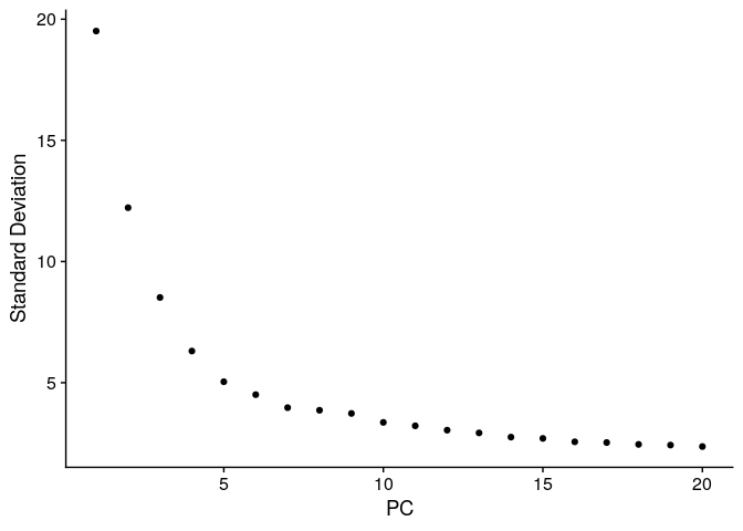
ElbowPlot(ser_integrated)
ser_integrated <- RunUMAP(ser_integrated, reduction = "pca", dims = 1:10) %>%
  FindNeighbors(.,dims=1:10) %>%
  FindClusters(.,res=c(0.3,0.5,0.7))
    ## 21:15:31 UMAP embedding parameters a = 0.9922 b = 1.112

    ## 21:15:31 Read 7528 rows and found 10 numeric columns

    ## 21:15:31 Using Annoy for neighbor search, n_neighbors = 30

    ## 21:15:31 Building Annoy index with metric = cosine, n_trees = 50

    ## 0%   10   20   30   40   50   60   70   80   90   100%

    ## [----|----|----|----|----|----|----|----|----|----|

    ## **************************************************|
    ## 21:15:32 Writing NN index file to temp file /tmp/Rtmp1pnHMW/file1b655befdec
    ## 21:15:32 Searching Annoy index using 1 thread, search_k = 3000
    ## 21:15:34 Annoy recall = 100%
    ## 21:15:34 Commencing smooth kNN distance calibration using 1 thread with target n_neighbors = 30
    ## 21:15:35 Initializing from normalized Laplacian + noise (using irlba)
    ## 21:15:35 Commencing optimization for 500 epochs, with 307598 positive edges
    ## 21:15:40 Optimization finished
    ## Computing nearest neighbor graph
    ## Computing SNN

    ## Modularity Optimizer version 1.3.0 by Ludo Waltman and Nees Jan van Eck
    ##
    ## Number of nodes: 7528
    ## Number of edges: 251352
    ##
    ## Running Louvain algorithm...
    ## Maximum modularity in 10 random starts: 0.9331
    ## Number of communities: 10
    ## Elapsed time: 0 seconds
    ## Modularity Optimizer version 1.3.0 by Ludo Waltman and Nees Jan van Eck
    ##
    ## Number of nodes: 7528
    ## Number of edges: 251352
    ##
    ## Running Louvain algorithm...
    ## Maximum modularity in 10 random starts: 0.9068
    ## Number of communities: 13
    ## Elapsed time: 0 seconds
    ## Modularity Optimizer version 1.3.0 by Ludo Waltman and Nees Jan van Eck
    ##
    ## Number of nodes: 7528
    ## Number of edges: 251352
    ##
    ## Running Louvain algorithm...
    ## Maximum modularity in 10 random starts: 0.8842
    ## Number of communities: 15
    ## Elapsed time: 0 seconds
Visualize integrated data #
colnames(ser_integrated@meta.data)
    ##  [1] "orig.ident"             "nCount_RNA"             "nFeature_RNA"
    ##  [4] "sample_id"              "sample_type"            "chemistry"
    ##  [7] "percent_mt"             "RNA_snn_res.0.3"        "RNA_snn_res.0.5"
    ## [10] "RNA_snn_res.0.7"        "seurat_clusters"        "nCount_SCT"
    ## [13] "nFeature_SCT"           "integrated_snn_res.0.3" "integrated_snn_res.0.5"
    ## [16] "integrated_snn_res.0.7"
# Notice the clustering results now have the preface "integrated"
# Instead of RNA

# A new assay is present called "integrated"
ser_integrated
    ## An object of class Seurat
    ## 52029 features across 7528 samples within 3 assays
    ## Active assay: integrated (2000 features, 2000 variable features)
    ##  2 other assays present: RNA, SCT
    ##  2 dimensional reductions calculated: pca, umap
ser_integrated@assays
    ## $RNA
    ## Assay data with 33694 features for 7528 cells
    ## First 10 features:
    ##  RP11-34P13.3, FAM138A, OR4F5, RP11-34P13.7, RP11-34P13.8,
    ## RP11-34P13.14, RP11-34P13.9, FO538757.3, FO538757.2, AP006222.2
    ##
    ## $SCT
    ## SCTAssay data with 16335 features for 7528 cells, and 2 SCTModel(s)
    ## First 10 features:
    ##  RP11-34P13.7, FO538757.2, AP006222.2, RP4-669L17.10, RP11-206L10.9,
    ## LINC00115, FAM41C, RP11-54O7.1, SAMD11, NOC2L
    ##
    ## $integrated
    ## SCTAssay data with 2000 features for 7528 cells, and 1 SCTModel(s)
    ## Top 10 variable features:
    ##  S100A8, S100A9, LYZ, GNLY, NKG7, CD74, HLA-DRA, CST3, FOS, CCL5
# View by chemistry and clusters
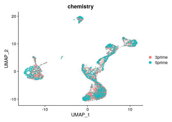
DimPlot(ser_integrated,group.by="chemistry")
DimPlot(ser_integrated,group.by="integrated_snn_res.0.3")
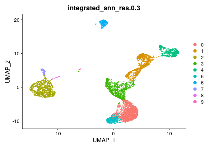
# View chemistry across clusters - much better
ser_integrated@meta.data %>%
  select(integrated_snn_res.0.3,chemistry) %>%
  table()
    ##                       chemistry
    ## integrated_snn_res.0.3 3prime 5prime
    ##                      0   1487    574
    ##                      1    696    535
    ##                      2    771    452
    ##                      3    764    456
    ##                      4    381    255
    ##                      5    335    223
    ##                      6    213    134
    ##                      7    124     26
    ##                      8     60      4
    ##                      9     33      5
Identifying DEGs #
Now that we have integrated the datasets, we can look for differentially expressed genes across the clusters.
It’s important to now switch back to the RNA assay. We do not want to use only the 2000 highly variable genes contained in the integrated assay to find differentially expressed genes.
DefaultAssay(ser_integrated) <- "RNA"
Idents(ser_integrated) <- "integrated_snn_res.0.3"

# Using logfc.thresold at 0.5 to speed this up
all_degs <- FindAllMarkers(ser_integrated,logfc.threshold = 0.5)
    ## Calculating cluster 0

    ## Calculating cluster 1

    ## Calculating cluster 2

    ## Calculating cluster 3

    ## Calculating cluster 4

    ## Calculating cluster 5

    ## Calculating cluster 6

    ## Calculating cluster 7

    ## Calculating cluster 8

    ## Calculating cluster 9
all_degs %>%
  group_by(cluster) %>%
  top_n(5,avg_log2FC) %>%
  arrange(desc(avg_log2FC))
    ## # A tibble: 50 × 7
    ## # Groups:   cluster [10]
    ##        p_val avg_log2FC pct.1 pct.2 p_val_adj cluster gene
    ##        <dbl>      <dbl> <dbl> <dbl>     <dbl> <fct>   <chr>
    ##  1 0               2.12 0.995 0.18  0         2       S100A8
    ##  2 0               2.04 0.993 0.265 0         2       S100A9
    ##  3 0               2.00 0.998 0.271 0         2       LYZ
    ##  4 3.27e-130       1.95 1     0.064 1.10e-125 9       JCHAIN
    ##  5 0               1.81 0.968 0.038 0         6       CD79A
    ##  6 0               1.78 0.93  0.036 0         2       VCAN
    ##  7 0               1.75 0.986 0.259 0         4       GNLY
    ##  8 1.67e-114       1.74 1     0.127 5.63e-110 8       HLA-DQA1
    ##  9 9.49e-182       1.73 0.947 0.038 3.20e-177 9       PLD4
    ## 10 0               1.73 0.953 0.078 0         2       FCN1
    ## # ℹ 40 more rows
Conclusions #
We have now walked through a method to integrate two datasets that have a known batch effect like chemistry. In practice, a batch effect can be anything from a patient specific sample to differences in how data was generated or differences in sequencing depth between samples.
Saving data #
# saveRDS(ser_integrated,file=paste(full_path,"PBMC_integration_final_output_231024.rds",sep=""))